Net2Plan [2, 8] is a free and open-source Java tool devoted to the planning, optimization and evaluation of communication networks. It has been originally thought as a tool to assist the teaching of communication networks design courses. Eventually, it has converted into a powerful network planning tool for the academia and industry, together with a growing repository of network planning resources.
Net2Plan is built on top of an abstract network representation, so-called network plan, based on seven abstract components: nodes, links, routes, traffic demands, protection segments, shared-risk groups and network layers. The network representation is technology-agnostic, thus Net2Plan can be adapted for planning networks in any technology. Technology-specific information can be introduced in the network representation via user-defined attributes attached to any of the abstract components mentioned above. Some attribute names has been fixed to ease the adaptation in well-known technologies (i.e. IP networks). For more information, see Section 3.1↓.
Net2Plan is implemented as a Java library along with both command-line and graphical user interfaces (CLI and GUI, respectively). The GUI is specially useful for laboratory sessions as an educational resource, or for a visual inspection of the network. In its turn, the command-line interface is specifically devoted to in-depth research studies, making use of batch processing or large-scale simulation facilities. In sum, Net2Plan is a tool intended for a broad spectrum of users: industry, research, and academia.
Regardless of the interface (CLI or GUI) selected by the user, Net2Plan currently provides four different tools:
Offline network design: Targeted to evaluate the network designs generated by built-in or user-defined offline network design algorithms, deciding on aspects such as the network topology, the traffic routing, link capacities, protection routes and so on. If needed, those algorithms based on constrained optimization formulations (i.e. ILPs) can be fast-prototyped using the open-source Java Optimization Modeler library (JOM [1]), to interface to a number of external solvers such as GPLK, CPLEX or IPOPT.
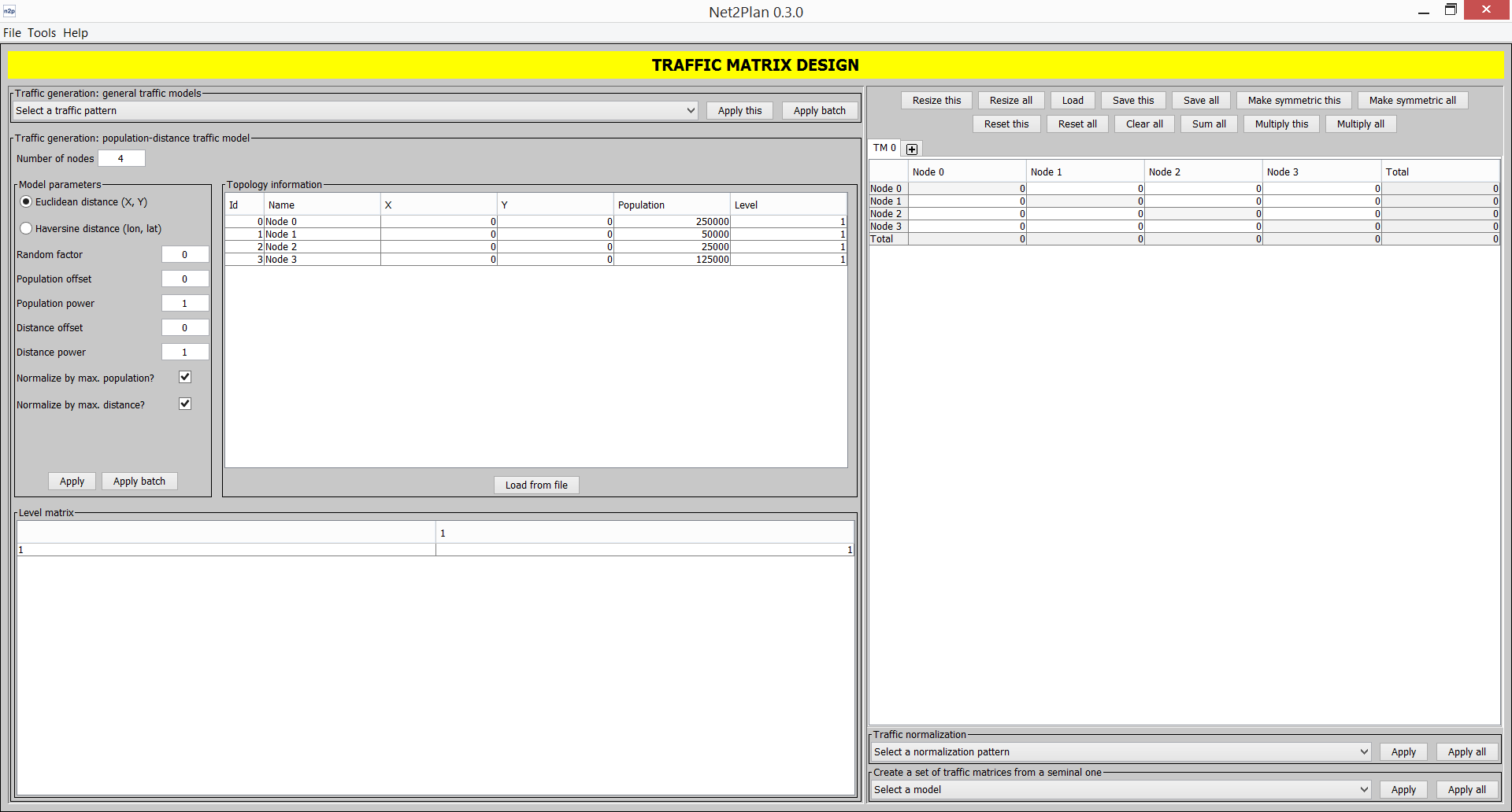
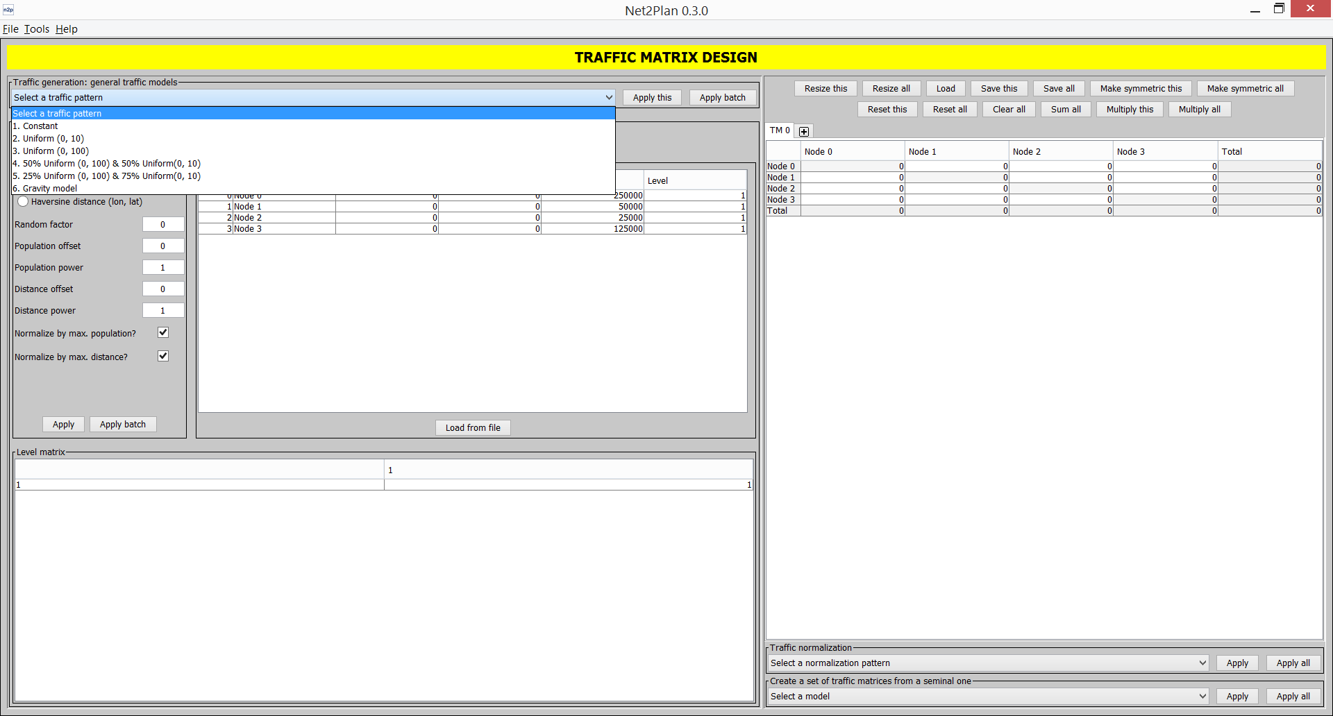
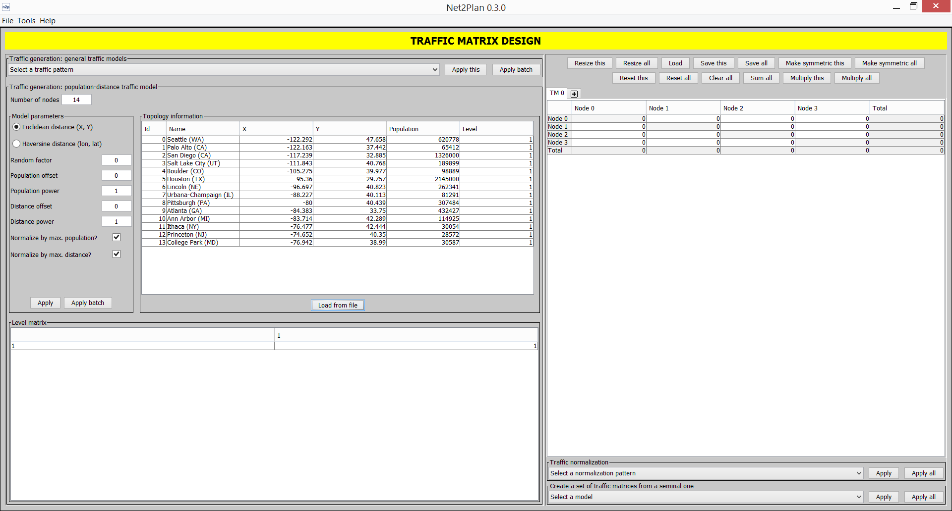
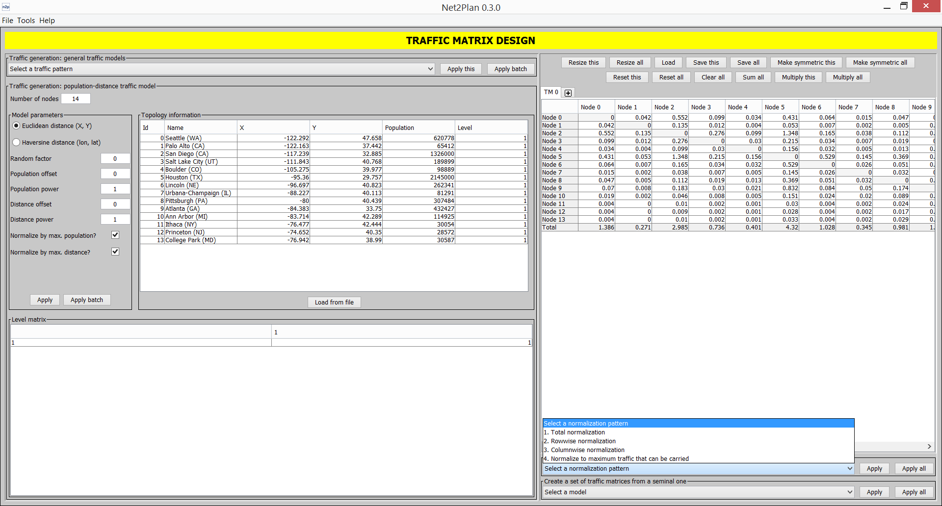
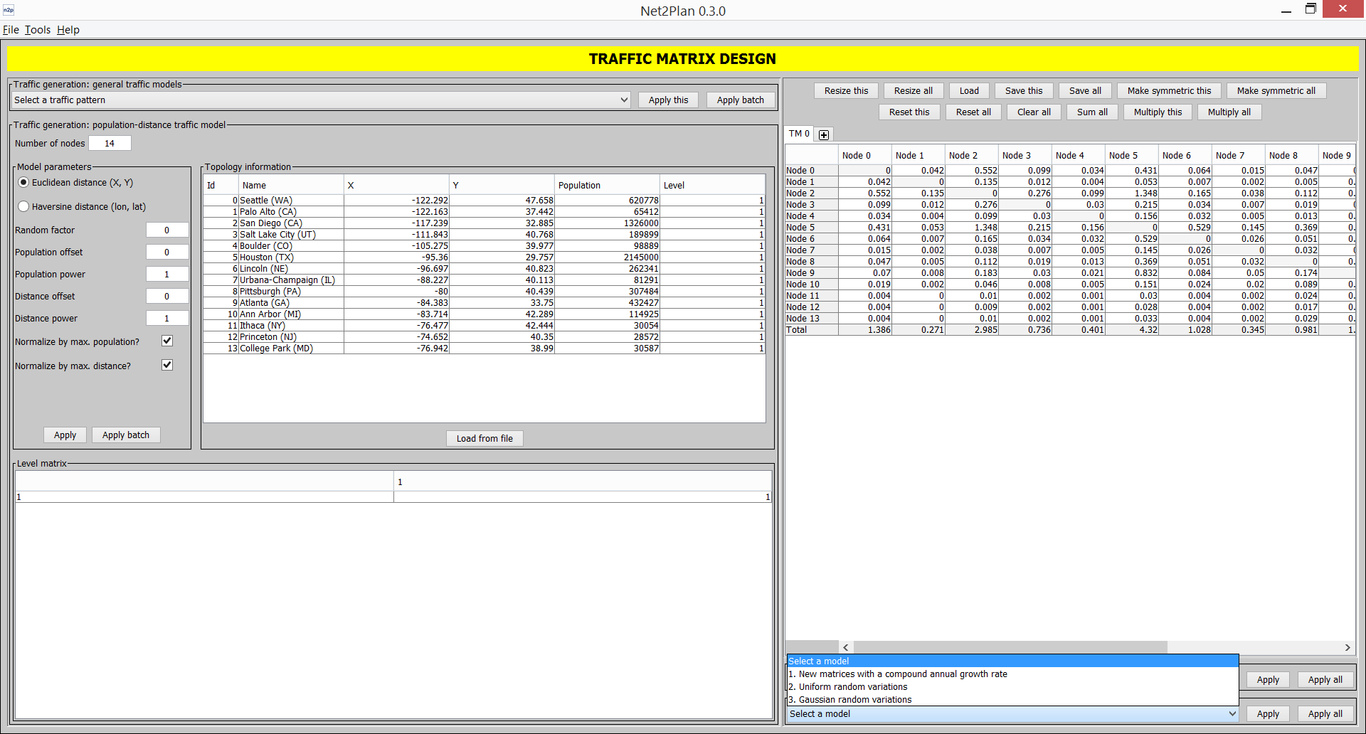
Traffic matrix generation: Assists users in the process of generating, normalizing and manipulating traffic matrices. Traffic matrix generation can be automated following several random models found in the literature, gravity model, etc. Traffic matrices can be normalized in different forms, e.g. so that the new matrices match a particular value of traffic in the nodes, or becomes an upper bound to the traffic a given network can carry In addition, it is possible to manually edit or automatically create variations to seminal traffic matrices (e.g. random variations, traffic forecasts according to compound-annual growths...).
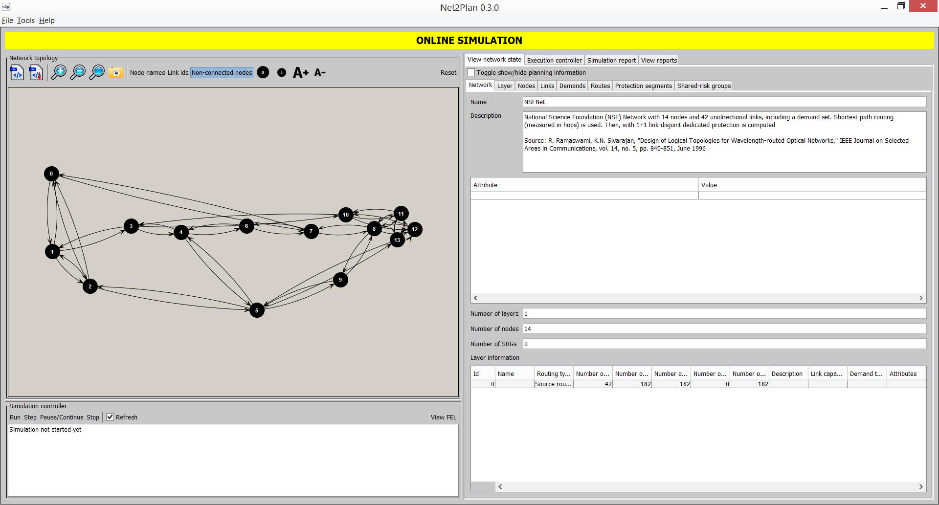
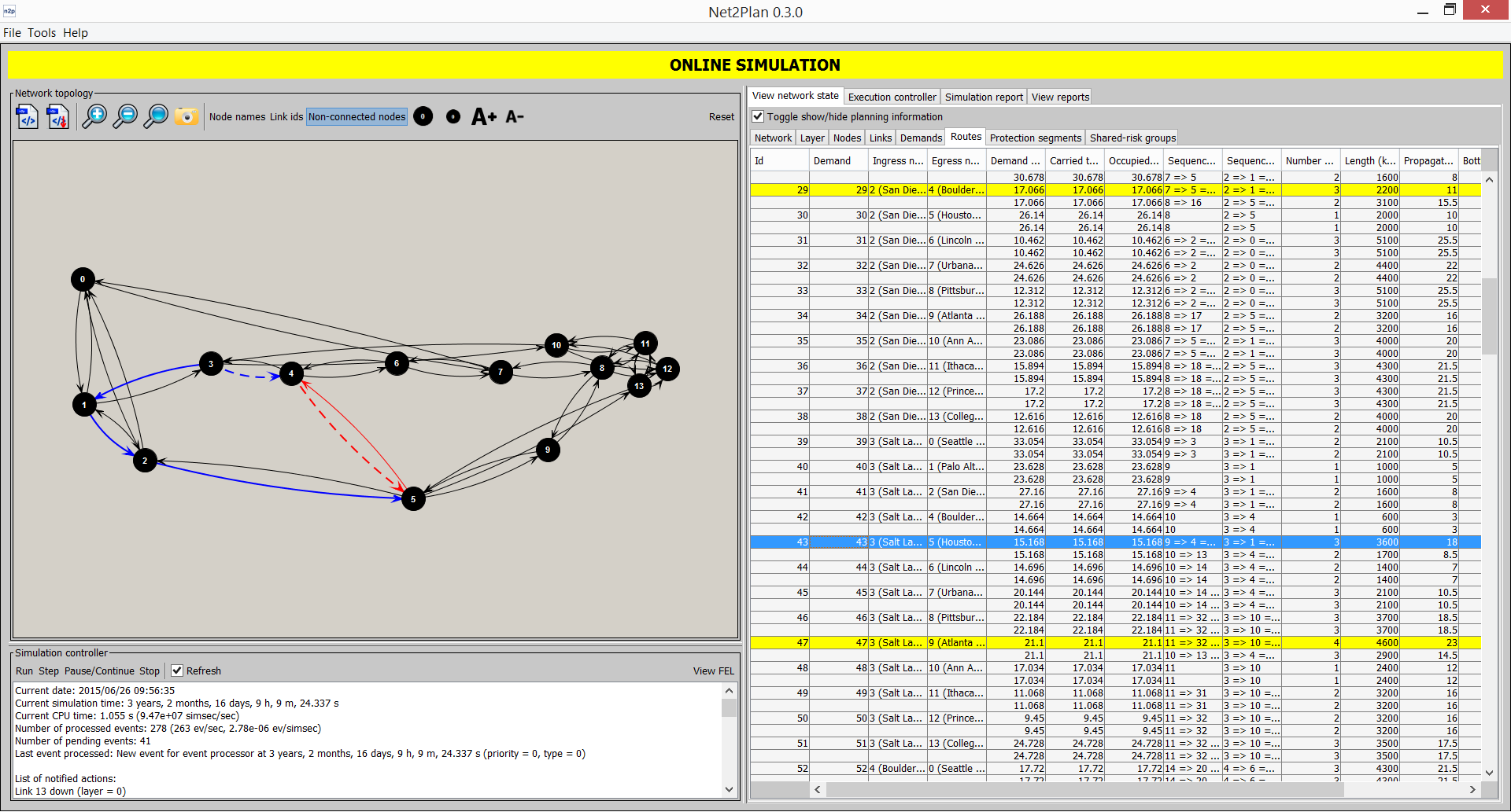
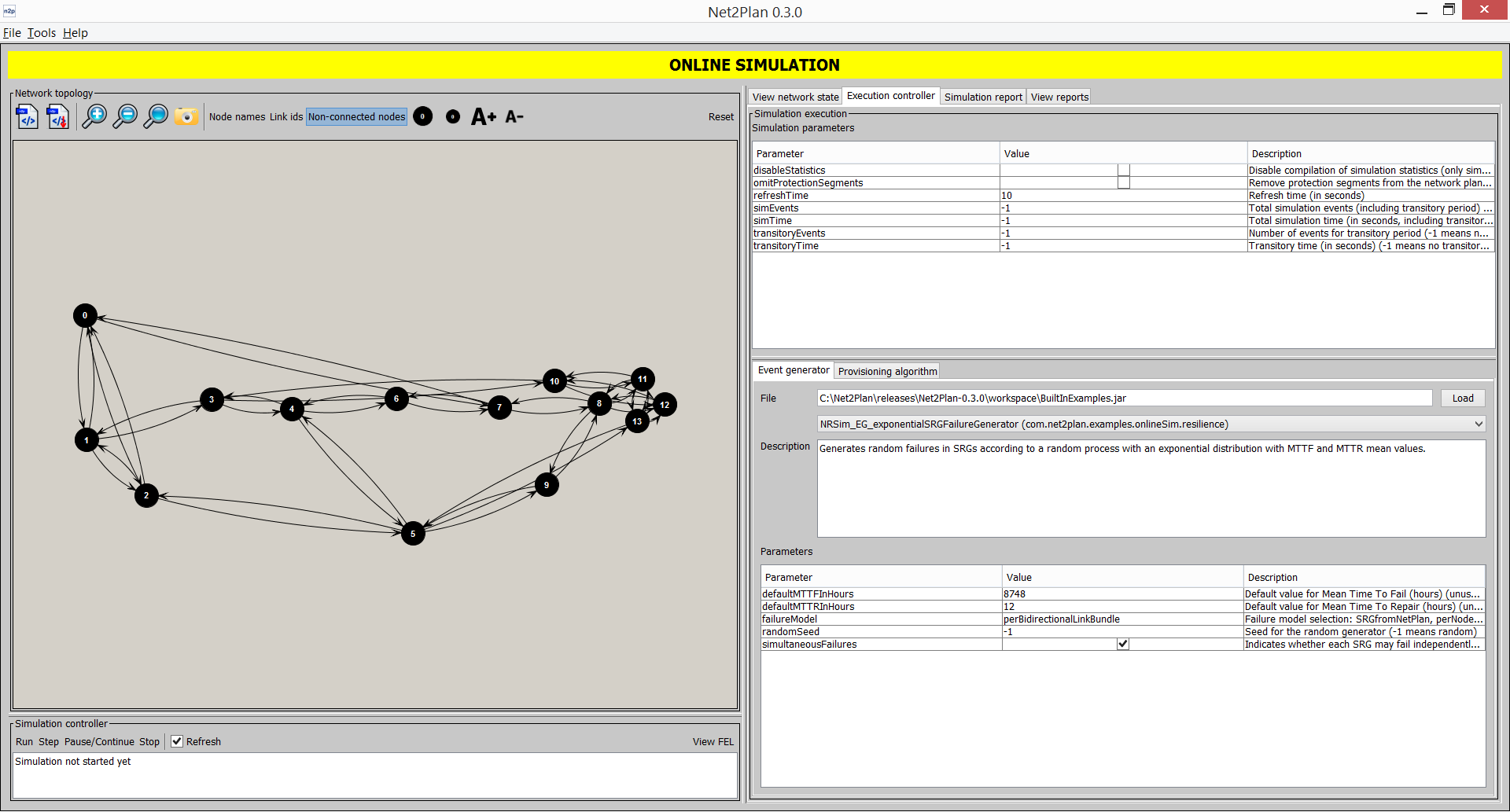
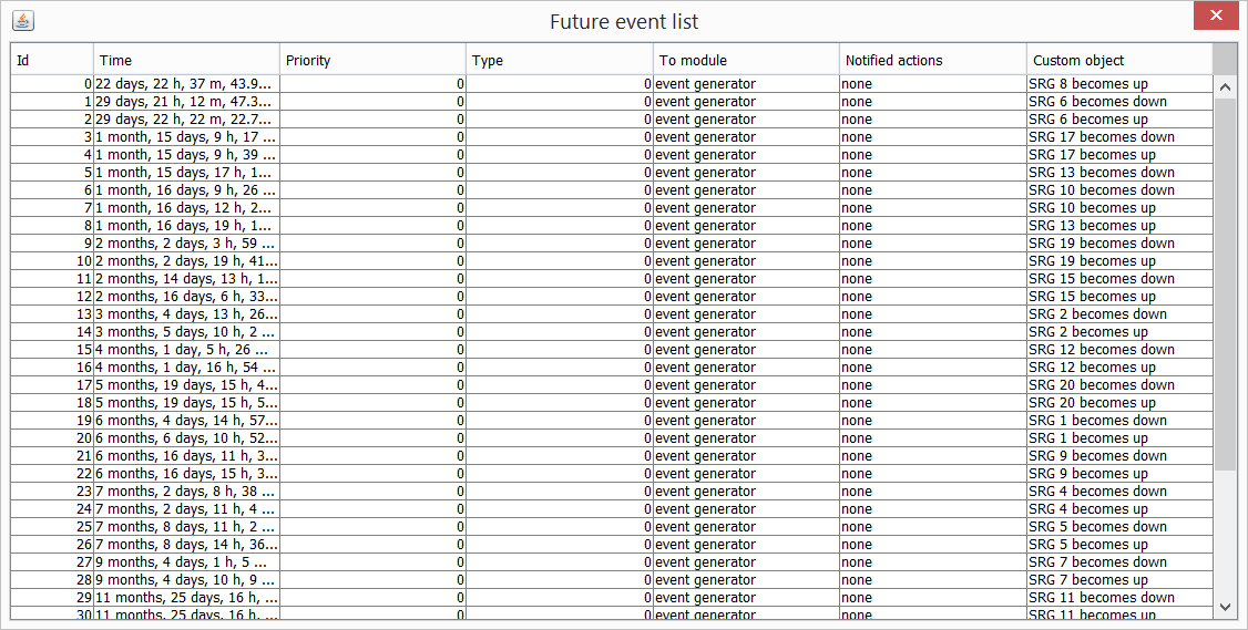
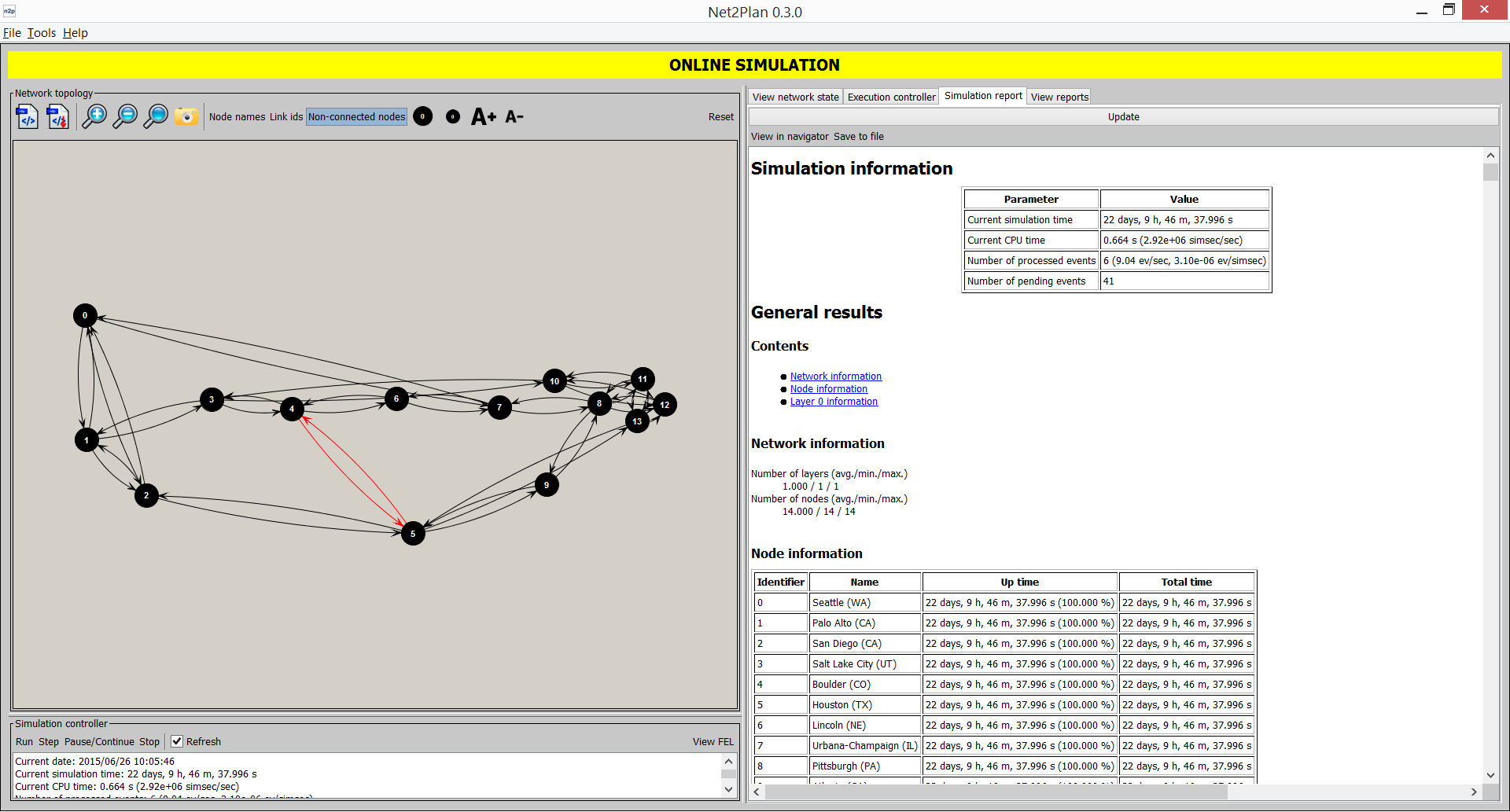
Online simulation: Permits the (joint) evaluation of network recovery schemes, connection-admission-control (CAC) systems, or dynamic provisioning algorithms for time-varying traffic. At the end of the simulation, some metrics (including either predefined metrics or custom ones) are presented.
Reporting: Net2Plan permits the generation of built-in or user-defined reports, from any network design. The report generation tool is integrated within all the previous functionalities, so that it is possible to create reports collecting performance measures in any of these aspects.
In all the features, the GUI organizes network statistics and performance estimations computed from the network design/simulation.
Algorithms in each of the features mentioned are Java .class/.jar files implementing a particular public interface (see Javadoc information). Net2Plan allows testing built-in or user-created algorithms. Creating a new algorithm for a particular Net2Plan feature, just requires programming a Java class implementing the appropriate interface.
And remember that Net2Plan is free and open-source! It is licensed under the GNU Lesser General Public License Version 3 or later (the “LGPL”).
Numerous network planning software tools can be found spanning a broad range of platforms, systems, languages, functionalities and applications. Some of them are oriented to the industry, whereas others are developed by academia for educational and research purposes. On the academia side, researchers investigating novel planning problems commonly need full control of the planning decisions, and develop their algorithms almost from scratch. Planning algorithms can be based on solving problem formulations (i.e. Integer Linear Programs) using specialized solvers (i.e. CPLEX, or MOSEK), or applying heuristic techniques. From the industry side, there is a trend to prefer commercial network planning tools that hide the planning decisions and any algorithmic details under intuitive graphical interfaces resembling computer-aided tools. All of them provide a more or less complete set of features to design and analyze networks, without relying on a specific vendor. These features are simulations of several configuration scenarios, routing schemes, network recovery tests, or traffic load analysis.
Unfortunately, existing tools lack of flexibility for testing different planning algorithms (e.g. users are only allowed to use built-in algorithms) or are not designed for educational purposes (e.g. their underlying algorithmic details are not publicly available). This is very important, since network optimization is more than drag and drop icons and connecting them to build a network. In addition, those tools only provide support for mature technologies and protocols for which there is a definite and large market, but don’t provide assistance for the abundance of possible prospective studies on emergent alternatives which could be performed.
In contrast, Net2Plan is a publicly-available open-source network optimization tool, not constrained to any specific network technology (and suitable to any of them), which allows users to test their own algorithms, or use the built-in ones. Net2Plan assists the task of creating and evaluating network design algorithms by providing a large set of built-in examples (together with its source code), many of them thoroughly described in the examples section of [2], a set of libraries (e.g. compute k-shortest paths, network performance metrics, or random traffic matrix models) documented in the Library API Javadoc (see Section 4.1↓ to know where you can find it). Moreover, automatic report generation (with built-in or user-defined reports) and post-analysis simulation tools integrated in Net2Plan help users to get insight into the network design merits.
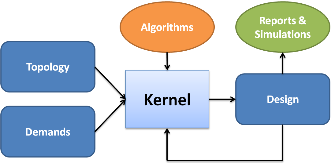
The Net2Plan philosophy enforces software reutilization. Once an algorithm is developed within the Net2Plan framework it can be modified or reused as parts of others, and can be applied to any network instance, so that network can be progressively designed. That is, users can chain successive algorithms, each one completing a part of the network design. For instance, you can start with a network where only the nodes are defined. Then, an algorithm is used to define the links in the network according to some figure of performance. Afterwards, another algorithm can be run to jointly decide on the capacity in the links and routing of the flows, for a given traffic matrix. As a result, Net2Plan can be a powerful tool for communications network planning courses, since students can see step by step how their designs grow. Besides, once the network design is completed, users can analyze and evaluate it by means of several reports, which can be built-in or user-defined ones, and post-analysis simulation tools. Fig. 2.1↓ summarizes this philosophy. In addition, the tool is intended to become a repository for network planning algorithms in any technology. Thus, the algorithms in the repository will become open for validation and verification, improving the trustworthiness of their results.
Figure 2.1 Workflow
In our opinion, all of these building blocks make Net2Plan a powerful tool for network planning for academia and industry.
As stated in the previous section, Net2Plan is designed with the aim to overcome the barriers imposed by existing network planning tools for two main reasons: (i) users are not limited to execute built-in algorithms, but also can integrate their own algorithms, applicable to any network instance, as Java classes implementing particular interfaces, and (ii) Net2Plan defines a multilayer network representation, so-called network plan, based on abstract concepts such as nodes, links, routes, traffic demands, protection segments, forwarding rules, shared-risk groups and network layers, without relying on any network technology. We believe that these are the key features enabling Net2Plan to be applicable to almost any (existing or not) technology, in contrast to the restricted scope of commercial tools, limited to mature technologies and built-in algorithms.
Nonetheless, even though Net2Plan is a technology-agnostic tool, users can introduce their technology-specific information via user-defined attributes for each element in the network design. However, Net2Plan provides some libraries (i.e. IPUtils, WDMUtils and FlexGridUtils) to ease the prototyping of some technology-specific algorithms. More detailed information can be found in Section 3.1.9↓.
The network design is stored into a data structure so-called network plan (class com.net2plan.interfaces.networkDesign.NetPlan in the Net2Plan library). In the offline network design feature, algorithms receive a network plan and return a modified network plan. The NetPlan object contains only the base minimum member variables (node position, link capacity, link length, offered traffic by demand...), which can be accessed or modified by getX() and setX() methods. Problem- or technology-specific or user-defined attributes, that are often attached to a network element (node, link...) in a specific tool, are stored in key-value maps within the NetPlan object. By doing so, users can add/remove attributes to every network element at run-time without having to change the NetPlan representation. For more information, check the Library API Javadoc for the class NetPlan.
Interestingly, this network representation applies to the offline network design tool as well as to the online simulation, instead of using different representations for each tool, providing a coherent and simple framework.
The network element represents the complete network. Thus, there is one and only one network element in each network representation. The network element is just a holder of general information that can be attached to the network. It has three member variables: name, description and attributes. Network name is a general string the user can define as a title of the network. Network description is also a string, that can be used to attach a short description to the network. Both are shown in the graphical user interface. Finally, the network attributes is an arbitraty set of name-value pairs that can be used to attach any arbitrary information to the network.
Operator networks are typically organized in multiple layers (i.e., service and transport layers, IP and optical layers, and so on), but commercial software has little or none multilayer capabilities. Net2Plan offers a flexible multilayer representation in which layers are entities containing links, demands, routes and protection segments and forwarding rules, while nodes and shared-risk groups are defined with a network-wide scope, that is, they appear in all layers. In order to provide a communication or coordination mechanism between layers, an integrated capacity approach [5] is implemented. The seminal concept behind this model is the following: an upper-layer link is considered to be realized by (or coupled to) a lower-layer demand, then the summation of carried traffic for such demand determines the capacity of the link at the upper layer. Hence, Net2Plan is able to cover a wide range of multilayer network scenarios and services, with an arbitrary number of layers coupled in arbitrary forms. Any network design is composed of, at least, one layer.
Layers are characterized by seven member variables: identifier, name, description, link capacity units, demand traffic units, routing type and attributes. The identifier is internally defined by the kernel and determines a serial unique number of the layer. Name and description sets general strings that the user can use for layer title and brief description, respectively. Link capacity units is an informational-only (it does not affect to any computation) string to indicate the units for the capacity of the links. In contrast, demand traffic units is an informational-only string to indicate the units for offered traffic. Routing type is used to determine the type of routing in the layer: source routing or explicit routing (see Section 3.1.6.1↓), and hop-by-hop routing (see Section 3.1.6.2↓). Finally, layer attributes are an arbitrary set of name-value pairs that can be used to attach any arbitrary information to the layer.
Important: To allow some kind of retrocompatibility with previous single-layer versions of Net2Plan, all the methods accessing to the NetPlan object are duplicated (but some of those refer to node and SRG properties, since they are network-wide elements not attached to any specific layer) so that the layer identifier can be omitted. Internally, the non-layered method calls to the layer method, using as layer identifier the one selected with the setLayerDefaultId() method. In the GUI, the default layer is the active layer. In constrast, in the CLI the default layer is the first-available layer. Users should take this into account if they are applying single layer algorithms to multilayer networks.
Nodes are the basic entity of a network design, and are either a connection point, a redistribution point or a communication end-point, which are able to send, receive, or forward traffic over a communication channel (or link).
Nodes are characterized by four member variables: identifier, position, name and attributes. The identifier is internally defined by the kernel and determines a serial unique number of the node. The node position sets the position of the node in a bidimensional Cartesian plane. The node name is a general string that is assigned to the node, e.g. to be shown in the graphical interface. Finally, node attributes are an arbitrary set of name-value pairs that can be used to attach any arbitrary information to the node.
Along with nodes, links comprise the topology of the network. They are the communication channels enabling connectivity between two nodes. In Net2Plan, links are unidirectional, from a node to another one. Two nodes can be connected by zero, one or more links. However, self-links (links where origin node and destination node are the same one) are forbidden.
Links are characterized by nine member variables: layer identifier, link identifier, origin node, destination node, capacity, length, propagation speed, coupled demand and attributes. Layer identifier is the serial number of the layer to which the link is attached. Again, the link identifier is a serial unique identifier of the link. Origin and destination nodes are the identifiers of the corresponding nodes. Capacity is the amount of traffic the link is able to carry. Link length (assumed to be in kilometers) and propagation speed (assumed to be in kilometers per second) represents the physical length and propagation speed of light in the link, respectively, to be used e.g. for propagation delay calculations. The coupled demand attribute is an optional attribute used to indicate a coupling relationship with a lower layer demand. Finally, link attributes are an arbitrary set of name-value pairs that can be used to attach any arbitrary information to the link.
Regarding to demand coupling, once a link is coupled to a demand, the link capacity is no more the defined value by the user, but the carried traffic of the coupled demand in the lower layer.
Traffic is modeled through a set of demands (or commodities). Each demand represents an offered end-to-end traffic flow to the network. In Net2Plan, demands are considered unicast, that is, they have only one ingress node and one egress node. In addition, self-demands are not allowed.
Demands have seven member variables: layer identifier, demand identifier, ingress node, egress node, offered traffic volume, coupled link and demand attributes. Again, layer and demand identifiers are unique serial number assigned by the kernel uniquely identifies the layer and the demand, respectively. The ingress node is the traffic source node identifier, while the egress node is the sink node identifier. The offered traffic volume is the traffic volume for the demand that is offered to the network. All, a part, of none of it can be actually carried (this information is given by the routes in the network). The coupled link attribute is an optional attribute used to indicate a coupling relationship with an upper layer link (if coupled, upper layer link capacity will be equal to the carried traffic of the demand). Finally, demand attributes are an arbitrary set of name-value pairs that can be used to attach any arbitrary information to the demand.
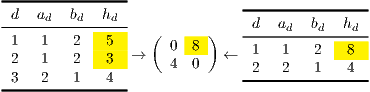
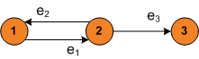
A simplified approach to model the offered traffic between nodes is the so-called traffic matrix. A traffic matrix is a matrix (where is the number of nodes in the network) in which each pair represents the (average) traffic from node to node . The main drawback of representing the offered traffic by means of traffic matrices, is that the traffic matrix representation assumes that at most one demand exists between each pair of nodes. Then, if we compute the traffic matrix representation of a demand set where some node pairs have more than one demand between them, an ambiguity can occur. This situation is posed in Fig. 3.1↓, where demands 1 and 2 from the demand set on the left are grouped in a single entry in the traffic matrix. The same result is obtained with the demand set on the right.
To provide a complete manner to model any form of traffic, the network representation of the offered traffic in Net2Plan is based on an arbitrary set of demands.
The routing model to represent how to get from a node to another one can be done in two basic ways. In source routing, all the information about how to get from here to there is collected at the source node, putting the traffic in end-to-end paths toward the destination ("there"). Instead, in hop-by-hop routing, the source is not expected to have all the information about how to get from a node to another one; it is sufficient for the source to know only how to get to the "next hop" (a node to which it has a link), and for that node to know how to get to the next hop, and so on until the destination is reached. As specified in Section 3.1.2↑, the network model allows using these two models in a per-layer basis.
Source routing is organized into two entities. Routes allows defining a set of paths, for each demand, able to carry traffic. To model pre-planned protection scenarios, a set of protection segments to reserve capacity in certain links in order to recover from eventual failures.
Routes
Routes are the paths in a network along which to send the traffic from demands. Routes are defined as an ordered (and contiguous) sequence of links going from the ingress node of the demand to the egress node, carrying a particular amount of traffic of the demand, and having zero, one or more protection segments associated to be used in case of failure. Each demand may have zero, one or more routes carrying traffic at the same time, provided that the carried traffic cannot overcome the offered traffic. Commonly, when each demand in the network have one single route associated, the routing is called unsplittable or non-bifurcated. Conversely, if at least one demand is carried by two or more routes, the network routing is referred as splittable or bifurcated. The traffic carried by each route can be any. Commonly, when all the routes in the network have an integer amount of traffic (or an integer multiple of a base quantity), the routing is called integral.
Routes have eleven member variables: layer identifier, route identifier, demand identifier, sequence of links, carried traffic, occupied capacity protection segment list, and route attributes. The layer identifier indicates the layer in which the route is established. The route identifier is a unique serial number determined by the kernel. The demand is the identifier of the demand associated to the path. The sequence of links is the ordered succession of link identifiers followed by the route. The sequence can contain loops. The only (natural) restriction is that one link should end in the node where the next starts, and the route should start and end at the demand ingress and egress nodes respectively. The carried traffic is the traffic volume that carries this route. However, the occupied capacity represents how much capacity is used in links to carry the traffic, allowing the user to model the effect of having different modulation formats in a link. This latter variable is optional, and if not specific, it will be equal to the carried traffic of the demand. The protection segment list is the ordered succession of protection segments that protect traffic from this route (see Section 2↓ for more information). Route attributes are an arbitrary set of name-value pairs that can be used to attach any arbitrary information to the route. Finally, note that during network operation routing can be modified, and the information of the original route would be lost. Hence, the original sequence of links, as well as the original carried traffic and occupied capacity are also stored.
Protection segments
A protection segment is defined as an ordered sequence of links with a specific volume of reserved capacity in each link. Protection segments are used to (partially or completely) protect one or more traffic routes, taking an alternative path to the original one when a failure occurs. The reserved bandwidth is taken from the capacity of the links. So the capacity of a link usable to carry traffic from the routes is the nominal link capacity, minus the reserved capacity of the protection segments traversing the link. Whereas loops are allowed for routes, they are forbidden for protection segments.
Protection segments are commonly used in conjunction with the NRSim_AA_genericProtectionAlgorithm, a built-in provisioning algorithm for network resilience simulation, that specifies a general form of reacting to nodes and links failures, making use of the protection segments defined in the network design. When a failure occurs, the NRSim_AA_genericProtectionAlgorithm processes the routes affected, and intends to reroute them making use of the associated protection segments. Information about the specific form in which NRSim_AA_genericProtectionAlgorithm reacts to failures and repairs is included in the Net2Plan algorithm repository in the web site.
Protection segments have five member variables: layer identifier, protection segment identifier, sequence of links, reserved capacity and protection segment attributes. Again, layer and protection segment identifiers are unique serial numbers determined by the kernel. The sequence of links is the ordered succession of links followed by the protection segment. A protection segment can only be assigned to a particular route, if the ending nodes of the protection segment are visited by the route. The reserved bandwidth member variable is the amount of bandwidth reserved in each of the traversed links. Finally, protection segment attributes are an arbitrary set of name-value pairs that can be used to attach any arbitrary information to the protection segment.
In conjunction with NRSim_AA_genericProtectionAlgorithm, protection segments become a mean to easily model many network protection schemes:
If a protection segment is associated to one single route, we model the so-called dedicated protection: the reserved bandwidth in that segment can only be used if the (primary) route fails. If a protection segment is associated to more than one routes, we are modeling a shared protection scheme.
If the reserved bandwidth of a protection segment is below the carried traffic by the primary route, you are modeling a partial-protection scheme.
If a protection segment shares the origin and destination nodes of the route, you are modeling a path-protection scheme. If only shares the origin and destination nodes of a link in the network, you are modeling a link-protection scheme. Otherwise, it is the subpath-protection scheme.
The users are encouraged to visit the specific documentation for modeling network recovery mechanisms using Net2Plan, available in the web site.
Hop-by-hop routing is implemented around the concept of forwarding rules. Essentially, forwarding rules are a generalization of destination-based routing in IP networks, in which the user is able to define, in a per-demand basis, the fraction of the total traffic entering a node how much is forwarded for each outgoing link. For instance, equal-cost multipath (ECMP) in IP networks evenly splits the traffic among the outgoing interfaces in the considered shortest paths. Using the forwarding rules, users may apply ECMP as well as any other arbitrary traffic distribution.
Forwarding rules
The forwarding rules represent the traffic splitting distribution in a node for each individual demand. Considering that a certain amount of traffic of a demand is entering into a node, each forwarding rule represents the fraction of traffic (splitting ratio) that will leave the node through the corresponding link. There is no limitation on the value of splitting ratio, considering that the sum must be at most equal to 1, so that no more than the 100% of traffic is forwarded. Note that if the sum is below 1, there may be traffic losses. Note that some rules can be omitted if the traffic does not reach the node where they are installed.
Forwarding rules have four member variables: layer identifier, a demand-outgoing link pair, splitting ratio and attributes. The layer identifier represents the layer in which the forwarding rule is installed. The demand-outgoing link pair is the identifier of the forwarding rule, indicating the demand for which the rule applies as well as the outgoing link for which the traffic would be forwarded. The node where the rule will be “installed” is discovered by the kernel from the link information. The splitting ratio represents the fraction of the whole traffic from the demand reaching the node and leaving it through the given outgoing link. Finally, forwarding rule attributes are an arbitrary set of name-value pairs that can be used to attach any arbitrary information to the forwarding rule.
A shared-risk goup (SRG) is an artifact to represent a particular risk of failure for the network that, if happens, creates a simultaneous failure in a particular set of links and/or nodes. For instance, a SRG can be associated to the risk of accidentaly cutting a particular conduct that holds the links between two nodes (e.g. one in each direction). If this cut occurs, the two links would fail simultaneously. Then, they would remain unavailable until a reparation of the damage is completed.
SRGs have five member variables: identifier, set of affected nodes, set of affected links, mean time to fail, mean time to repair and SRG attributes. The SRG identifier is a unique serial number assigned by the kernel. The set of affected nodes contains the identifiers of those nodes that simultaneously fail when the risk associated to the SRG happen. Identically, the set of affected links contains the identifiers of the links. Note that both nodes and links fail simultaneously. The mean time to fail is the expectation of the time (in hours) from the moment the failure is repaired until the moment it happens again. The mean time to repair is the expected time (in hours) from the moment the failure occurs until it is repaired. Finally, SRG attributes are an arbitrary set of name-value pairs that can be used to attach any arbitrary information to the SRG.
SRGs are used to model the failure risks that threat the network, and eases the design and evaluation of the network to adequatelly recover from these failures. As an example, SRG information can be used read in the online simulation tool to generate the failure/reparation events to which the provisioning algorithms should react. Also, the availability calculation and the disaster-vulnerability built-in reports (see Built-in Examples in [2]), that numerically estimates network availability measures (i.e. without simulation), make use of the SRG information.
In order to evaluate network resilience mechanisms, the network model allows setting ’up’ or ’down’ flags to nodes and links, using the setXXXUp() and the setXXXDown() methods in the NetPlan object, affecting to the traffic routing. Note that network reactions to a failure are problem-dependent, hence they must be appropiately implemented by users in their algorithms.
When a node or link becomes down, all the associated traffic is affected. As a convention, node and link failures are independent, that is, a node failure does not affect to its outgoing or incoming links, and they are considered as up, provided that the traffic will not be carried since the node is down. The kernel is able to understand these circumstances and criteria, and it makes the computations accordingly.
In source routing, routes becomes also down, removing their carried traffic from metrics, but not from the route configuration, that is, if users call the getRouteCarriedTraffic() still returns the route carried traffic. Protection segments are also affected by failures, and also may become down. However, the reserved capacity by them remains reserved along all the link path, irrespective of the protection segment status. Due to the problem-dependent nature of some reaction algorithms, whenever all the resources (nodes and links) of a route or protection segment become up, routes and protection segments are kept as down and they must be restored to up using the setXXXUp() (for one or more specific routes or protection segments) or setAllXXXUp() (for all the routes or protection segments whose resources are all up).
In hop-by-hop routing, the forwarding rules are never modified under a failure/reparation event. The kernel internally does not consider the forwarding rules affected by a failure, and recomputes routing and metrics accordingly. Upon reparation, the kernel then reconsiders them again to restore the routing. In other words, the kernel applies the same forwarding rules to the surviving topology to make the routing. If users want a different mechanism, i.e. apply OSPF/ECMP over the surviving topology, then they should prepare an algorithm.
Due to the nature of the multilayer representation in Net2Plan, where upper layer links are seen as traffic demands in the lower layer, we use a capacity updating model under the consideration of the link capacity in the upper layer will be equal to the carried traffic of the lower layer demand [5]. Esentially, when some resources fail at a layer affecting some demands, this is seen by the associated upper link layers as a capacity reduction. However, the upper layer links are kept as up and, therefore, they may become oversubscribed since it will “carry” traffic in capacity-reduced links. As a consequence, failures do not propagate to higher layers, since the links directly affected by a lower layer failure are not aware of such failure, the upper layer demand routing is not affected, and layers above this layer are not affected. Note also that network reactions to multilayer failures (i.e. a node failure with associated links in multiple layers) depend on the problem-specific requirements, e.g. in a 2-layer network rerouting the traffic in the lower layer to restore upper layer capacity or reroute directly in the upper layer. Hence, users should develop their own reaction algorithms tailored to their problems.
As stated in previous sections, the NetPlan object contains only the base minimum member variables (node position, link capacity, link length, offered traffic by demand...). Problem- or technology-specific attributes that any algorithm wants to define and handle (i.e. link weights in an algorithm for routing design in IP/OSPF networks), should be stored using the key-value attribute maps within the NetPlan object. Then, algorithms can add/remove attributes to every network element at run-time without having to change the NetPlan representation. For more information, check the Library API Javadoc for the class NetPlan.
As an example, let us to suppose you are using an algorithm to determine link capacities given a traffic demand set, and you have to choose between several capacity values in order to minimize the total network cost while all traffic is carried. You could define the options for capacity values and associated costs into two network-wide variables which would be used by your algorithm.
Important: All key-value pairs in the attribute maps are stored as String values. Users are responsible to make the proper conversions. For example, you can store an int array as a succession of numbers separated by spaces.
In the Technology Conventions section on the website, users can find some examples of technological conventions used within Net2Plan, and supported by the library API. By the way, users are free to use their own conventions, without support from the library API.
Table 3.1↓ summarizes the aforementioned information. Here, if a member attribute cannot be change by the user once the element is defined, or if the attribute is internally handled by the kernel, is marked as read-only.
Element
Member attribute
Description
Network
name
Network name
description
Network description message
attributes
Arbitrary name-value pairs attached to the network
Layer
id
Identifier (read-only)
name
Network name
description
Network description message
capacity units
Link capacity units
traffic units
Demand traffic units
routing type
Routing type: source routing or hop-by-hop routing
attributes
Arbitrary name-value pairs attached to the layer
Node
id
Identifier (read-only)
name
Node name
position
Position in a 2D plane (x,y)
attributes
Arbitrary name-value pairs attached to the node
Link
layer
Layer identifier (read-only)
id
Identifier (read-only)
origin node
Origin node of the link (read-only)
destination node
Destination node of the link (different than the origin node) (read-only)
capacity
Capacity of the link
length
Physical link length (in kilometers)
propagation speed
Propagation speed (in kilometers per second)
coupled demand
(Optional) Lower layer and demand identifiers
attributes
Arbitrary name-value pairs attached to the link
Demand
layer
Layer identifier (read-only)
id
Identifier (read-only)
ingress node
Source node of the demand (read-only)
egress node
Sink node of the demand (different than the ingress node) (read-only)
offered traffic volume
Amount of traffic offered by the demand
coupled link
(Optional) Upper layer and link identifiers
attributes
Arbitrary name-value pairs attached to the demand
Route (source routing)
layer
Layer identifier (read-only)
id
Identifier (read-only)
demand
Demand identifier (read-only)
sequence of links
Sequence of links (and protection segments) followed by the route
carried traffic
Amount of traffic carried by the route (in demand units)
occupied capacity
Occupied capacity in links by the route (in link capacity units)
original sequence of links
Sequence of links followed by the route in the original state
original carried traffic
Amount of traffic carried by the route (in demand units) in the original state
original occupied capacity
Occupied capacity in links by the route (in link capacity units) in the original state
backup segment list
Set of protection segments associated to the route
attributes
Arbitrary name-value pairs attached to the route
Protection segments (source routing)
layer
Layer identifier (read-only)
id
Identifier (read-only)
sequence of links
Sequence of links followed by the protection segment
reserved capacity
Amount of bandwidth reserved in every link in the protection segment (in capacity units)
attributes
Arbitrary name-value pairs attached to the protection segment
Forwarding rule (hop-by-hop routing)
layer
Layer identifier (read-only)
id
Identifier (read-only)
demand
Demand identifier (read-only)
outgoing link
Outgoing link identifier (read-only)
splitting ratio
Fraction of the demand traffic entering the node and going through the outgoing link
attributes
Arbitrary name-value pairs attached to the forwarding rule
SRGs
id
Identifier (read-only)
affected nodes
Set of identifiers of nodes affected by the failure
affected links
Set of identifiers of links affected by the failure
mean time to fail
Average time in hours between failure reparation and next failure to occur
mean time to repair
Average time in hours between failure and failure reparation
attributes
Arbitrary name-value pairs attached to the SRG
Table 3.1 Summary of network elements involved in Net2Plan, and its member attributes
One of the most important features of Net2Plan is that it allows users to execute their own code (algorithms, reports... in general we refer to them as runnable code). Here, we briefly describe how to integrate users’ code into Net2Plan.
Runnable code is implemented as Java classes, using single .class files or integrated into .jar files, with a given signature:
Algorithms for offline network design should implement the interface com.net2plan.interfaces.networkDesign.IAlgorithm.
Reports should implement the interface com.net2plan.interfaces.networkDesign.IReport
Reaction algorithms that react to network events (e.g., used in the online simulation tool, and some reports), should implement the interface com.net2plan.interfaces.simulation.IEventProcessor Modules that generate events to be consumed by reaction algorithms should implement the com.net2plan.interfaces.simulation.IEventGenerator interface.
A complete information of each interface can be found in the Library API Javadoc. Integration of runnable code simply requires saving it into any directory of the computer, although it is a good practice to store them in the workspace directory of Net2Plan.
In addition, in order to improve the user experience, kernel is able to catch any exception thrown by runnable code, and print exception messages in the Java console. Recall that any information printed to the Java console by any runnable code (e.g., exception messages, and also any messages printed on purpose into System.out) , is accessible from Net2Plan (see Section 5.1.1.3↓). This is a valuable resource for debugging the algorithms executed in Net2Plan. In particular, messages from exceptions include a full trace of the error (files, line number of the exception...).
When the runnable code wants to stop its execution raising an exception that needs to be informed to the user in a more clear form (not through the Java console), we recommend to throw the Net2PlanException class (see Library API Javadoc for more information). The message associated to this exception is printed in a pop-up dialog instead of the Java console, and thus is more visible to the user. For instance, let us assume an algorithm that receives an input parameter from the user, that should be positive. A good programming practice is starting the algorithm checking if the received parameters are within their valid ranges. If a negative number is received as the input parameter (or something that is not a number), it is better to raise a Net2PlanException that shows the information message in a pop-up in Net2Plan, than a general Java RuntimeException whose message can be read only if the user checks the Java console.
Important: When runnable code is implemented as a Java .class files, the full path to the class must follow the package name of the class, in order to successfully load the code. For example, if we create an algorithm named testAlgorithm in the package test.myAlgorithms, the full path to the class must be like ...{any}.../test/myAlgorithms/testAlgorithm.class. For .jar files there is not any restriction on the full path, they can be stored at any folder.
Important: Net2Plan allows to make “online” changes in the runnable code, that is, users can modify their runnable code, recompile and reexecute it (just clicking the “Execute” button at the graphical interface) without the need to restart Net2Plan.
3.2.1 Net2Plan Library, Built-in Examples and Code Repository
Net2Plan assists the task of creating and evaluating algorithms by providing built-in example algorithms and a set of libraries (e.g., k-loopless shortest paths, minimum spanning tree…). An exhaustive list of built-in algorithms and the Library API Javadoc can be found in [2]. Net2Plan web site is expected to become a valuable repository for network planning algorithms. The algorithms in the repository will be open for validation and verification, improving the trustworthiness of planning results.
The library is divided into three parts:
Input/Output interfaces: Provides a set of classes and interfaces for the different tools: offline network design, reporting and simulators.
Libraries: Provides a set of useful libraries to develop algorithms and reports (i.e. to compute candidate path list, graph metrics...)
Utils: General utility static methods for Java language (i.e. methods to work with int/double arrays)
For more information, we refer to the Library API Javadoc.
Often, some network design problems are solved by modeling them as optimization problems (i.e. integer linear problems, linear problems, convex problems…), and then calling an optimization solver to obtain its numerical solution. In this context, optimization modeling tools are targeted to ease the definition of the problem decision variables, constraints and objective function, and become an interface with the (usually complex) solver libraries. AMPL and GAMS are examples of commercial modeling tools. JOM (Java Optimization Modeler) is an open-source Java library developed by Prof. Pablo Pavón Mariño, which can interface with a number of solvers using vectorial MATLAB-like syntax, which i.e. permits the addition of sets of constraints in one line of code. Current JOM version can interface with GPLK (free) and CPLEX (commercial) solvers for mixed integer linear problems, and IPOPT (free) for non-linear differentiable problems. JOM directly interfaces with compiled solver libraries (.DLLs in Windows and .SOs in Linux), via Java Native Access (JNA). JOM is independent from Net2Plan and can be used for any type of optimization problem. However, Net2Plan uses JOM in all the network design algorithm examples based on solving formulations that are included in the Net2Plan distribution [1].
In Appendix A↓, we include a brief summary of mathematical notation we use in the built-in code using JOM library. Also, in Appendix B↓, we include the mathematical definition of several performance metrics integrated into Net2Plan.
3.2.3 Preparing a Java IDE for Net2Plan programming
For users interested in integrating their own algorithms to Net2Plan, it is required to prepare the Java IDE to program the runnable code. Essentially, users only have to configure their preferred Java IDE to use Java 7 (or later), and to include the libraries in the lib folder (see Section 4.1↓) within the Net2Plan distribution in the Java build-path. In Eclipse, the latter can be done in the option Project => Properties => Java Build Path => Libraries => Add External JARs... In Netbeans, the option can be found in Run => Set Project Configuration => Customize => Libraries => Add JAR/Folder... Additionally, Javadoc and sources can be attached using the corresponding options in the IDEs. Once the Java IDE is configured, users can start programming their own Net2Plan code.
In the website, there is a videotutorial section in which users can see examples of algorithm’s integration, where Java IDE preparation is also addressed.
4 Installation guide, system requirements and starting Net2Plan
Net2Plan requires Java Runtime Environment 7 or higher versions and a screen resolution of, at least, 800x600 pixels. Since it is developed in Java, it works in the most well-known operation systems (Microsoft Windows, Linux, Mac OS X).
To install Net2Plan, just save the compressed file in any directory. Then, extract all the files and folders into a new directory, for example C:\Work\Net2Plan (in a Windows environment), and now it is ready to run.
To execute Net2Plan in GUI mode (see Section 5↓), just double click on Net2Plan.jar, or execute the following command in a terminal: java -jar Net2Plan.jar
To execute Net2Plan in CLI mode (see Section 6↓), execute the following command in a terminal: java -jar Net2Plan-cli.jar
Important: Net2Plan is tightly coupled with the Java Optimization Modeler (JOM) library, already shipped with Net2Plan, in order to execute some included network designed algorithms based on optimization models. Please, follow the instructions in the JOM website to install the solvers.
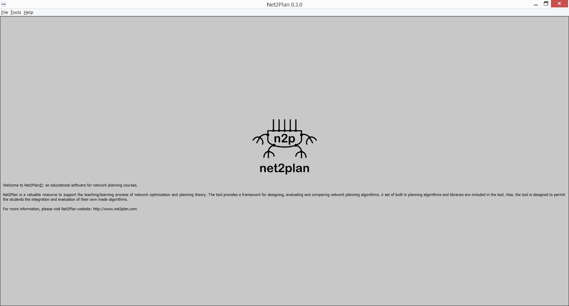
To start Net2Plan in GUI mode double click on Net2Plan.jar, or execute the following command in a terminal: java -jar Net2Plan.jar. The welcome screen will appear.
Figure 5.1 Welcome screen
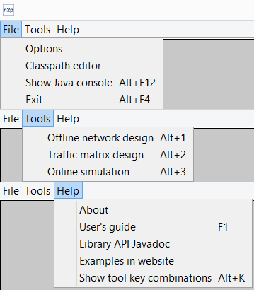
In the top menu (see Fig. 5.2↓) you can choose among the different options which Net2Plan provides. Below are listed and explained:
File menu: Provides access to general configuration and debugging functionalities
Tools menu: Provides access to the set of applications developed for Net2Plan: Offline network design, Traffic generation, and Online simulator
Help menu: Provides access to the help documentation of Net2Plan and return to the welcome (about) screen
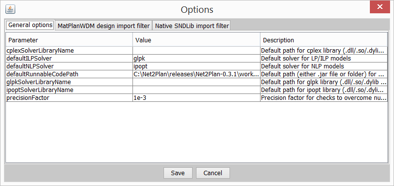
Use Options to set Net2Plan-wide parameters. These options have a global scope to all Net2Plan modules: are used within the kernel, and, for instance, to compute delay metrics in built-in reports. Users implementing their own algorithms/reports/event generators/event processors have access to these parameters through a key-value map attached as an input parameter so-called net2planParameters. For more information, see the class com.net2plan.interfaces.networkDesign.Configuration in the Library API Javadoc.
In this version the general configurable options are:
precisionFactor: Precision factor for checks to overcome numeric errors. Default: 1e-3. This parameter allows considering in the kernel small tolerances in the sanity-checks of the network designs. It avoids situations in which numerical inaccuracies (e.g. caused by finite precision of the solvers) would be interpreted as errors. For instance, if an algorithm returns a design where the traffic carried by a link is 10.0000001 and link capacity is 10, the kernel may show a warning. The precision factor applies since the actual check performed has a margin given by the precision factor. Default value of precisionFactor is , and its value is constrained to be in range (0,1).
defaultRunnableCodePath: Default path that will be used by tools in the GUI as the first option to load external code (i.e. algorithms). It can be either a .jar file or a folder. Default value is the BuiltInExamples.jar included within Net2Plan.
Users can configure other options related to the use of JOM library within Net2Plan:
defaultILPSolver: Default solver to be used for solving Linear Programs (LP) or Mixed Integer Linear Programs (MILP). Default: glpk.
defaultNLPSolver: Default solver to be used for solving Non-Linear Programs (NLP). Default: ipopt.
cplexSolverLibraryName: Default path for cplex library (.dll/.so file). Default: None
glpkSolverLibraryName: Default path for glpk library (.dll/.so file). Default: None
ipoptSolverLibraryName: Default path for ipopt library (.dll/.so file). Default: None
Important: Default solvers are only used for internal operations requiring a solver. External algorithms from users, or even built-in examples may have their own solver-related parameters. Regarding to solver library names, they are used if, and only if, an algorithm specifies two solver-related parameters, solverName (i.e. cplex) and solverLibraryName (i.e. cplex125.dll), and the solver library name is empty. Otherwise, the non-empty default value for the algorithm will be used by default.
Important: External plugins may require some configuration, which will appear in the form of additional tabs.
Options are saved when user presses the “Save” button. Then, new values are checked and saved in the options file.
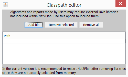
Although a moderate library set is provided within Net2Plan, users may require extra Java libraries (.jar files) to develop their own algorithms or reports (i.e. mathematical or graph theory libraries). So, the classpath editor avoids the tedious task of include Java libraries in environment variables (i.e. CLASSPATH in Windows).
Important: In the current version of Net2Plan Java libraries can be included in run-time, but unfortunately it is not possible to do the same to remove libraries. In this case, user is forced to restart Net2Plan.
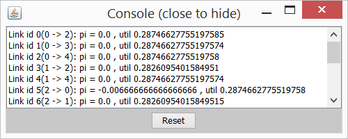
This feature centralizes the error handling within Net2Plan. When an error is thrown, for example, due to invalid input parameters in an algorithm, the error and the stack trace is shown there. Moreover, System.out/System.err is redirected there also, allowing users to debug their Java code. The console can be accessed also using the combination ALT+F12.
Figure 5.5 Error console
Important: Due to limitations in Java Virtual Machines, when JNI/JNA for native library access is used, the native output (i.e. stdout in C/C++) is not equivalent to the Java output, thus such an information will not appear in the Java error console. A workaround is to start the GUI from the command-line according to the instructions given in Section 4↑.
This menu organizes the tools provided within Net2Plan: Offline network design, Traffic matrix design and Online simulation. These tools are described in their own sections.
This tool assists users in the process of offline network design and planning. In practical network design different variables can be involved: network nodes, network links, link capacities, the traffic routing, the traffic demand... Usually, offline network design problems receive some of this information as input parameters (e.g. traffic demand, and network topology) and try to optimize others (e.g. capacities in the links and traffic routing) according to a performance merit of interest. Clearly, the number of possible variants and subtypes of network design problems is infinite. Moreover, different technologies add their own particular aspects to network design. For this reason, network design has become a mixture of art and engineering.
In an attempt to provide a (somehow) systematic criteria to cathegorize network design problems, in Net2Plan documentation and repository we adopt the following naming scheme, which is just an extension of the network design problems’ taxonomy in Kleinrock’s book [7]:
Topology Assignment (TA): Decides on the nodes and/or links in the network.
Capacity Assignment (CA): Decides on the capacities in the links are decision variables to optimize.
Flow Assignment (FA): Decide on the routing of the traffic demands over the network links .
Bandwidth Assignment (BA): Decide on the traffic volume to be carried by each demand
According to this naming scheme, combinations of these problems are named merging the acronyms. For example, a capacity and flow assignment (CFA) problem involves the joint computation of routing and link capacities. We remark that this taxonomy should be considered as an attempt to give a didactic organization to the utmost diversity of planning problems that arise in communication networks.
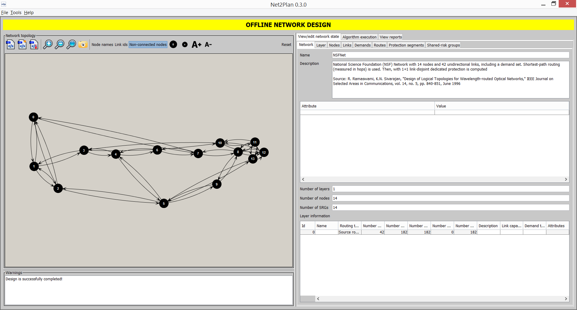
Selecting Offline network design opens the Network design window (or ALT+1), which you can use to create a static or offline network design. A network design in Net2Plan is a com.net2plan.interfaces.networkDesign.NetPlan object, containing anetwork representation comprising the elements described in 3.1↑: network nodes, links, traffic demands, routes, protection segments and SRGs. The word offline here means that all the variables in the network plan are supposed to be deterministic values, that also do not change along time. For instance, offered traffics are assumed to be constants representing the average traffic volumes, although in reality the traffic can fluctuate around this average in according to statistical patterns.
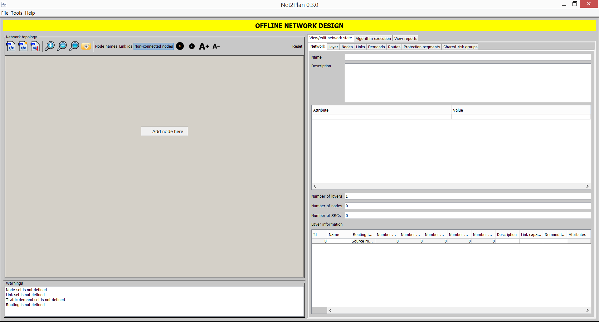
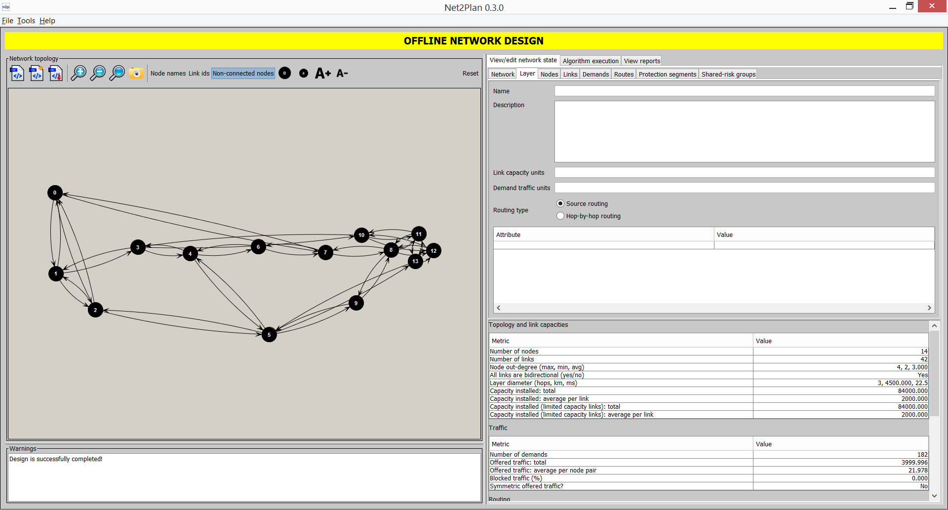
The workspace of the window is divided into three areas: input data, execution and reporting (right area), plot area (top-left area), and warning area (bottom-left area). In Net2Plan, network designs can be completed incrementally, modifying the current network design, that the user can inspect visually in the “Network Topology” panel, and the “Edit network plan” tab. When the offline design tool starts, the current network design is empty. Then, the user can modify it (i) using manual editions in the “Network Topology” panel or the “View/edit network state” tab, (ii) loading existing designs and/or traffics demands, (iii) applying offline design algorithms (that take the current network design, and return a modified design which becomes the current design).
This panel shows graphically the current network design, and permits modifying some parts of it. Users are able to add or remove nodes and links, zoom out and zoom in (and reset zoom), save a screenshot of the currently shown topology (in PNG format), and also show the name of the nodes and link identifiers. When the show non-connected nodes option is disabled, nodes without outgoing or incoming links will be hidden from the view. When a multilayer design is loaded, a combobox appears to allow users selecting the current layer.
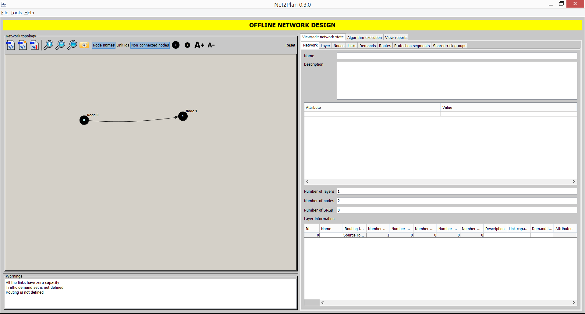
Nodes are inserted by right clicking into the canvas and using the option Add node here. Nodes can be removed by right clicking on them and using the option Remove node. Also it is possible to move nodes by dragging them (in this case, you must press CTRL key during that process).
Figure 5.8 Inserting a node
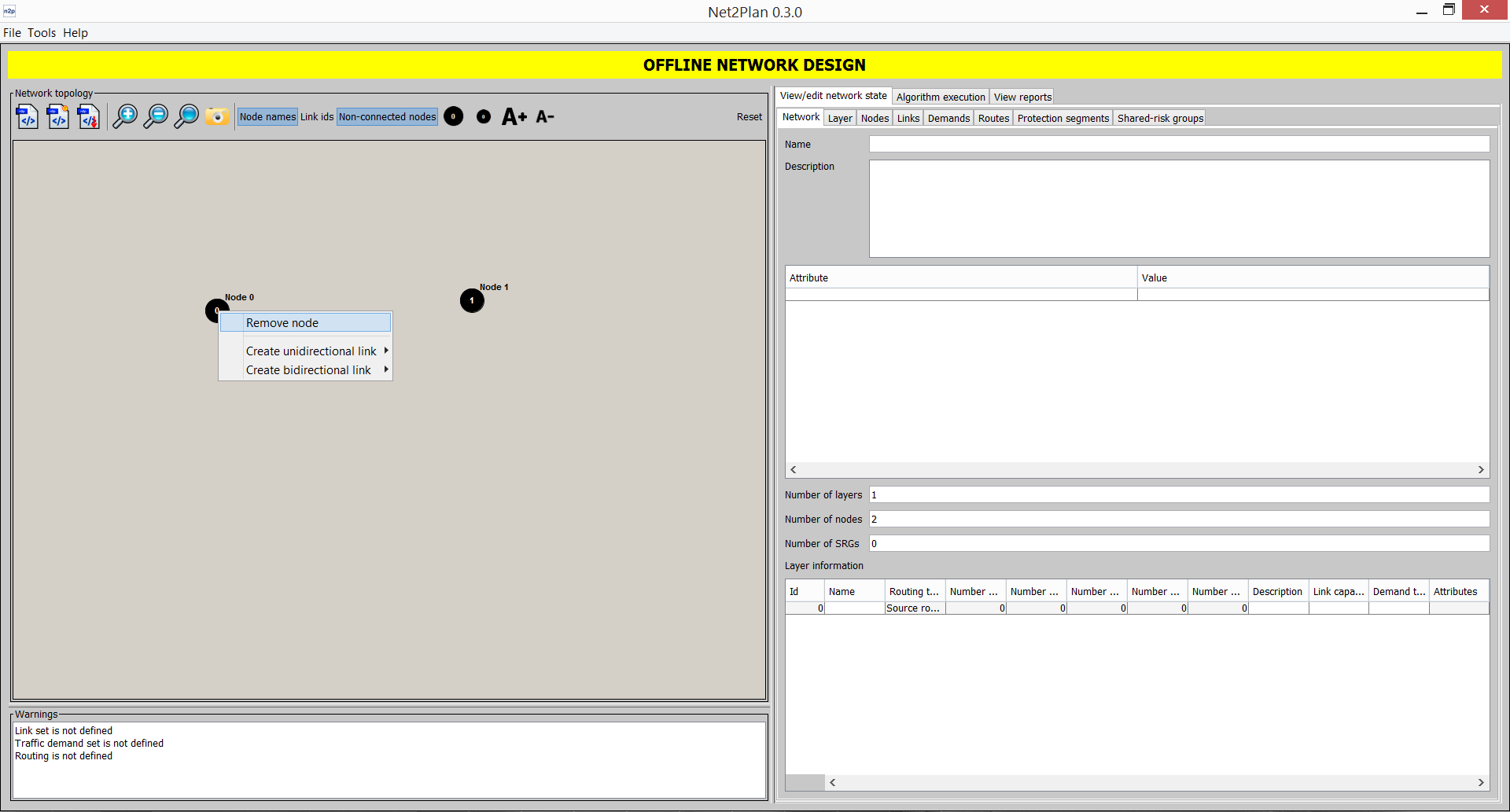
Links are inserted by clicking first in the origin node and then in the destination node. It is possible to insert unidirectional links or bidirectional ones (in this latter case, the user must press SHIFT key during that process). Also links can be inserted by right clicking over the origin node and selecting the destination node in the popup menu.
Figure 5.9 Inserting a link graphically
Figure 5.10 Inserting a link using a popup menu
The icons at the Network Topology panel permit (left-to-right):
First button loads a network design from a .n2p file. Loaded design becomes the current network design, previous design is lost.
Second button loads a .n2p file, but only extracting the set of offered demands from it (ignoring any other information). The loaded traffic demands replace the set of demands in the current network design, and leaves unchanged the rest of the current network design. Typically, the loaded file was generated using the Traffic matrix design functionality. If the number of nodes in the loaded file and the current network design are different, the operation is not completed and an error message is shown.
Third button saves current design into a .n2p file.
Fourth and fifth buttons are devoted to zoom-in and zoom-out, respectively, whereas the sixth one is to zoom-all.
Seventh button allows to take a snapshot of the canvas and save it to a .png file.
Eighth button toggles between showing or not node name.
Ninth button toggles between showing or not link identifiers.
Tenth button toggles between showing or not non-connected nodes.
Next buttons are used to increase/decrease node and font sizes, to enhance visualization.
Finally, the Reset button erases the current network design, which becomes an empty design
In this panel you can see some short messages of warning about the current network design e.g. if node, link or demand sets are defined, if routing is defined or not, if all the offered traffic is routed or there are traffic losses, and so on. No warning messages means that the current network design has nodes, links and offered traffic, that is routed without losses in the network, so that no link is oversubscribed (is supposed to carry more traffic than its capacity).
The “View/edit network state” (accessible with CTRL+1) tab shows complete information about the current network design, including some basic statistics and warnings that permit to visually fast-check the design and its performances. Also, this tab permits completing some simple modifications in the design, like adding/removing any element (layers, nodes, links, demands, routes, protection segments, forwarding rules and SRGs), setting the capacity of links, the offered traffic of demands, or the carried traffic of the routes. The “View/edit network state” tab is organized in nine sub-tabs, one for each type of element that comprises a network design in Net2Plan: Network, Layer, Nodes, Links, Demands, Routes, Protection segments, Forwarding rules and Shared-risk groups. When layer routing is source routing, Routes and Protection segment tabs are shown, but the Forwarding rules tab is hidden. When layer routing is hop-by-hop routing, the Forwarding rules tab is shown, and the other two are hidden. In general, fields coloured in gray are not editable, since they show information calculated from other base fields. Right-clicking in the sub-tabs provide fast-access to some element-related specific actions.
Figure 5.11 Edit network plan tab
Network
This tab shows statistical information describing the current network design at a network level (see Section 3.1.1↑).
Name, Description and Attributes: Shows the network name, description message, and set of user-defined key-value parameters associated to the Network element in the design. Right-clicking in the Parameters panel pemits adding/removing/editing attributes.
Number of layers, nodes and SRGs: These three (read-only) fields indicate the number of these elements in the network.
Layer information: This panel shows basic information about all the layers in the network such as name, description, link and demand units, attributes, and number of items for each layer-dependent element (links, demands, and so on). Here users can add/remove layers by right clicking on the table and using the corresponding option.
Layer
This tab shows statistical information describing the current network design at a layer level (see Section 3.1.2↑).
Name, Description, Link capacity units name, Demand traffic units name and Attributes: Shows the layer name, description message, link and capacity units, and set of user-defined key-value parameters associated to the Layer element in the design. Right-clicking in the Parameters panel pemits adding/removing/editing attributes.
Routing type: Allows setting the routing type of the layer between source routing and hop-by-hop routing. Note that users may change between them, and the kernel automatically will translate a routing into the other one. Source routing can be always translated into hop-by-hop routing. However, the other situation is not always possible. If forwarding rules are bad defined, i.e. traffic gets trapped into a loop, their equivalent routes cannot be found.
Topology and link capacities: This panels shows information characterizing the topology of nodes and links. The total number of nodes and links is just a count of these quantities. The maximum, minimum and average node out-degree is the max/min/average number of outgoing links of a node. The network diameter is the maximum shortest path distance between any node pair, where the distance is measured in hops, km and miliseconds. The link length in km is obtained from the NetPlan object (getLinkLengthInKm() method). The link propagation delay in seconds, converted to miliseconds later on, is obtained from the NetPlan object (getLinkPropagationDelayInSeconds() method). The conversion from km to miliseconds applies the propagationSpeedInKmPerSecond attribute of the link (getLinkPropagationSpeedInKmPerSecond() method) parameter. The total capacity installed sums the capacities in all the links (as they are stored in NetPlan object).
Traffic: This panel shows information characterizing the offered and (if exists) carried traffic in the network. If current design has no offered traffic, this panel is empty. The number of demands is just a count of this quantity. The total offered traffic sums the demand volumes. The average traffic per node pair divides the previous quantities by being the number of nodes in the network. The “is symmetric” field indicates whether or not the offered traffic is symmetric: if for every demand from node A to node B, exists a demand from B to A with the same volume. The percentage of blocked traffic is the fraction of the offered traffic that is not routed.
Routing: This panel shows information characterizing the routing of the traffic, and is empty if the design contains no routes. The number of routes is just a count of the number of route entries in the NetPlan object. The routing is qualified as bifurcated if at least one demand has two associated routed carrying traffic. Network congestion value with reserved bandwidth is the highest ratio between the occupied bandwidth (summing carried traffic and reserved bandwidth by protection segments) and the link bandwidth, among all the network links. The value without reserved bandwidth does not consider the bandwidth occupied by the protection segments. If the design has no protection segments, both values are equal. The average route length is the sum of the route distance (in number of hops, km or miliseconds) weighted by the fraction of the route carried traffic respect to the total amount of carried traffic in the network. Its meaning is the average distance followed by a fraction of traffic (e.g. a packet in packet-switched networks), chosen randomly. The field “Routing has loops?” prints “no” if all the routes are loopless (do not traverse any node more than once), and prints “yes” otherwise. In hop-by-hop routing, only network congestion and routing loops information are shown.
Resilience information (only source routing): This panel shows information that characterize the protection scheme defined in the design. The number of protection segments field is just a count of the number of protection segment entries in the NetPlan object. The average link capacity reserved for protection in % sums the reserved bandwidth by the protection segments among all the links, and divides it by the total capacity installed in the network links. The three next fields show the type of protection that receive the carried traffic. These percentages are computed as follows. Let a route have a carried traffic of . If the route has no associated protection segment, then the amount is considered unprotected traffic. If has one protection segment associated with a reserved bandwidth of at least , so that this segment is not associated to any other route, then the amount is considered a traffic with complete and dedicated protection. If does not fit into the previous definitions, sums as a traffic with partial and/or shared protection. The number of SRGs is a count of the number of SRGs defined in the NetPlan object. SRG definition characteristic observes if the SRGs defined follow one of some typical arrangements: one SRG per node, one SRG per unidirectional link, one SRG per unidirectional link bundle (all the links in the same direction together), one SRG per bidirectional link bundle (all the links between a node pair in the same SRG), or none. Finally, the % of routes protected (from the total defined routing, irrespective of the carried traffic) with SRG disjoint segments.
Figure 5.12 Layer view
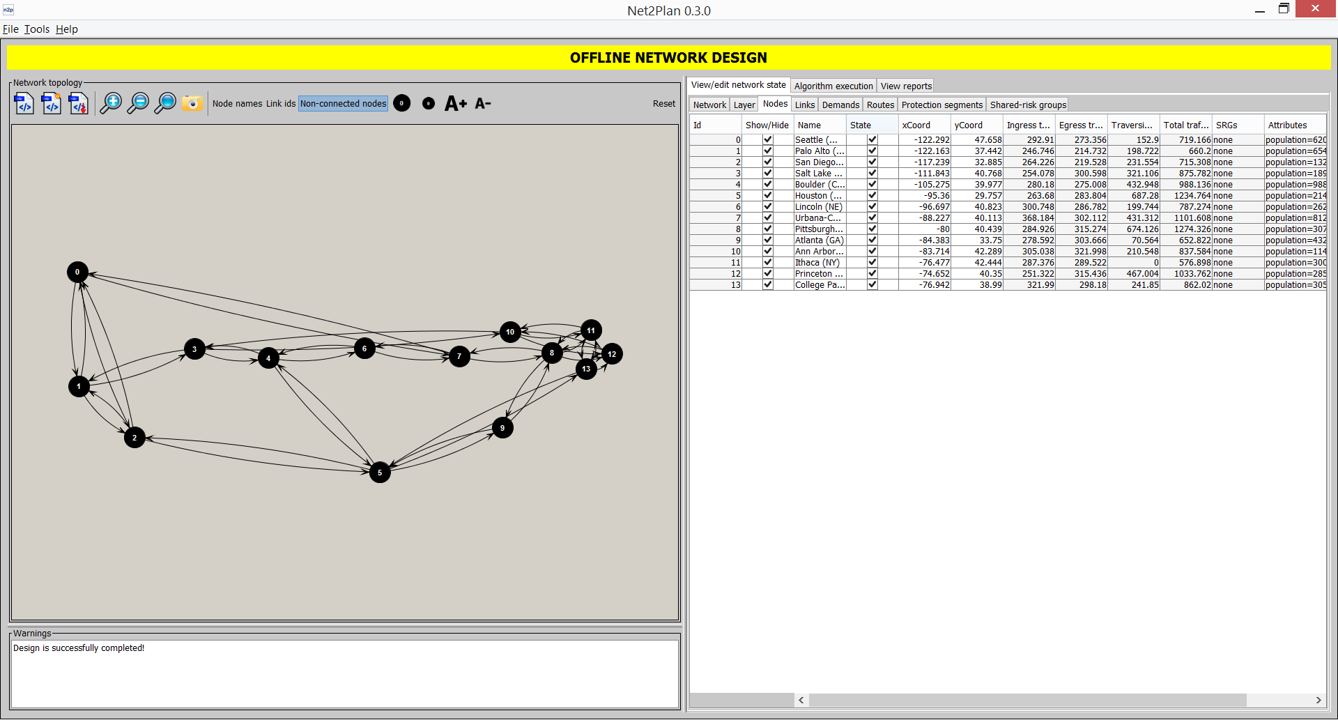
Nodes
This sub-tab shows the information related to network nodes (see Section 3.1.3↑). Clicking on each node highlights it in the left panel. Right-clicking in the panel provides several options as adding or removing nodes. Node Id is a serial number starting from 0 identifying the node. Node name, a user-defined string. xCoord and yCoord are the node X and Y coordinates to plot them in a map. Ingress and egress traffic is the sum of the carried traffic incoming to and outgoing from the node respectively. Traversing traffic is the carried traffic that enter the node, but is not targeted to it. The total traffic is the sum of previous three quantities. SRGs are the SRG identifiers that include the node. Finally, the last column shows the user-defined key-value attributes attached to the node. The two additional options allows showing/hiding the nodes and setting them as up/down, respectively. Note that the Show non-connected nodes option, when disabled, has priority over the setting in the Nodes tab. The up/down option allows users to play with the network to see the effect, in terms of traffic losses, of a failure. We would like to remark, as mentioned in Section 3.1.8↑, that the network does not react to failures i.e. rerouting traffic, and this can be done by algorithms. When nodes are again up, all associated routing is restored. Nodes in down state are highlighted in red in the topology view.
Figure 5.13 Nodes view
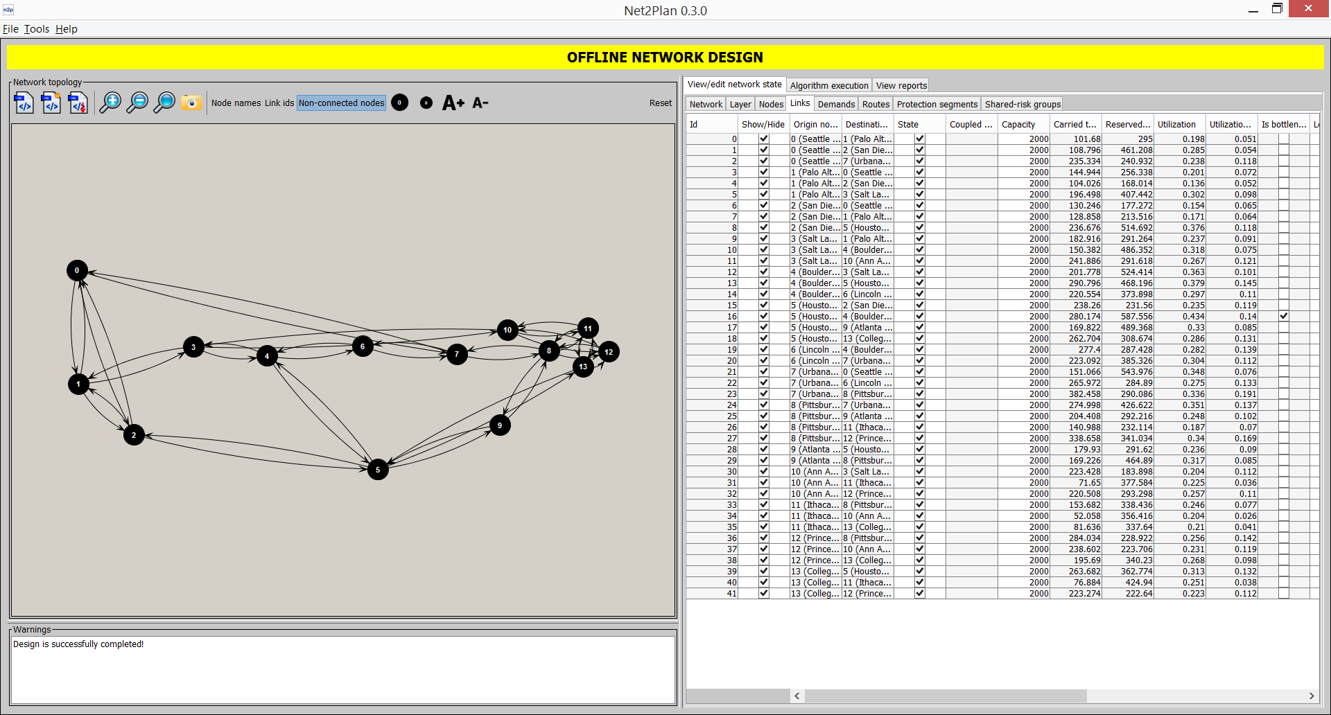
Links
This tab shows the information related to network links (see Section 3.1.4↑). Clicking on each link highlights it in the left panel (only if its node is not hidden). Link Id is a serial number starting from identifying the link. Link origin and destination nodes are the node identifiers of the link ends. Link capacity column shown the link capacity. Carried traffic sums the total amount of bandwidth that is occupied by the carried traffic of the routes traversing the link. Reserved for protection sums the total amount of bandwidth reserved by the protection segments traversing the link. Utilization is the fraction of link capacity occupied by the carried traffic plus the reserved for protection. Link length in km is the lengh of the link. Commonly, this value is equal to the euclidean distance between the link end nodes, but any other non-negative value could be stored. The number of routes counts the number of routes that traverse the link. The check box Is bottleneck is checked in the link (or links) that have the highest utilization in the network. Finally, the last column shows the user-defined key-value attributes attached to the link. The fields capacity, length and attributes are directly editable by the user in this panel. Right-clicking in the panel provides several options as adding or removing links, or setting the same attribute to all the links. Again, there are two options to play with link visibility and up/down state, where the same rationale than for the nodes applies.
Figure 5.14 Links view
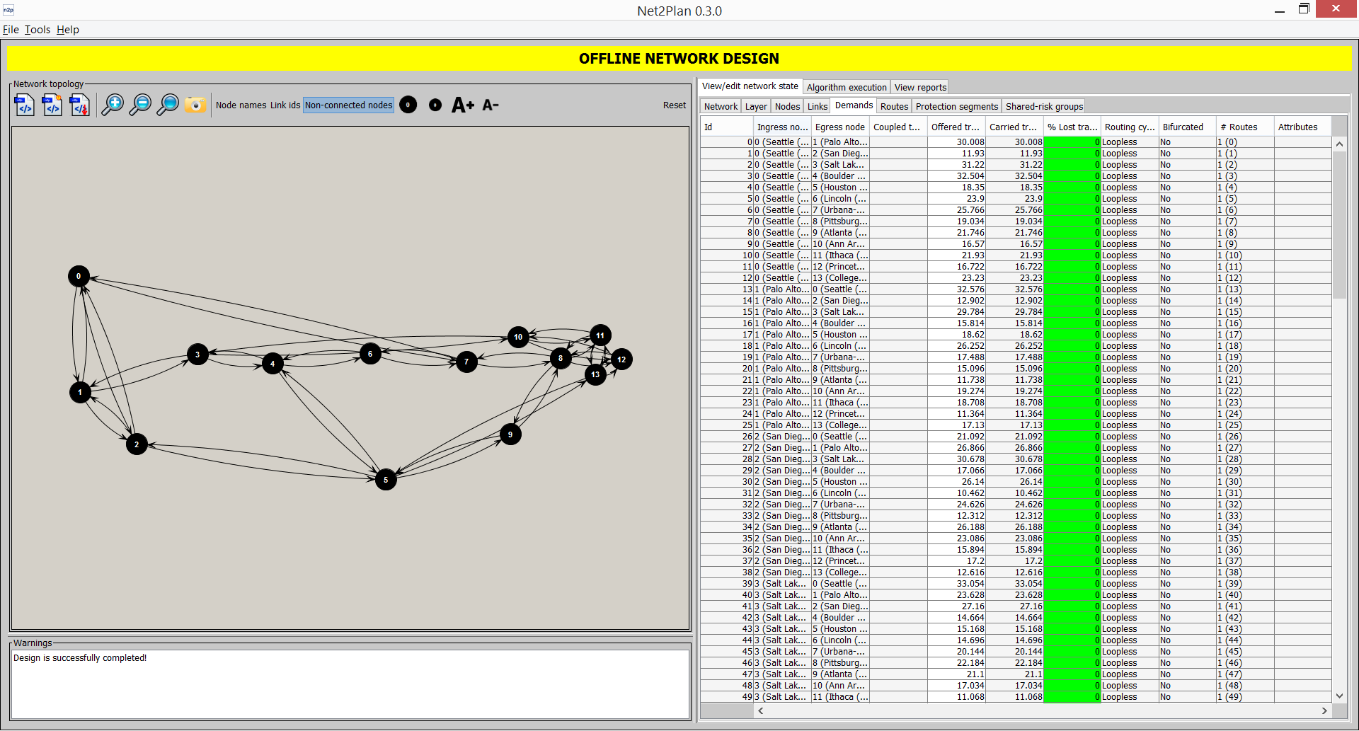
Demands
This sub-tab shows the information related to traffic demands (see Section 3.1.5↑). Clicking on each demand highlights its associated ingress and egress nodes in the left panel. Demand Id is a serial number starting from 0 identifying the traffic demand. Ingress node and Egress node are the initial and ending nodes of the demand. The offered traffic is the traffic volume offered, while the carried traffic is the amount actually carried by the routes associated to the demand. Lost traffic is the percentage of the offered traffic that is not carried. Note that if the demand has no associated routes, 100% of the offered traffic is lost. The column Bifurcated shows a “yes” is the demand routing is bifurcated i.e. the demand has two or more associated routes with carried traffic. The #Routes column indicates the number of routes and route identifiers associated to the demand. Finally, the last column shows the user-defined key-value attributes attached to the demand.
Figure 5.15 Demands view
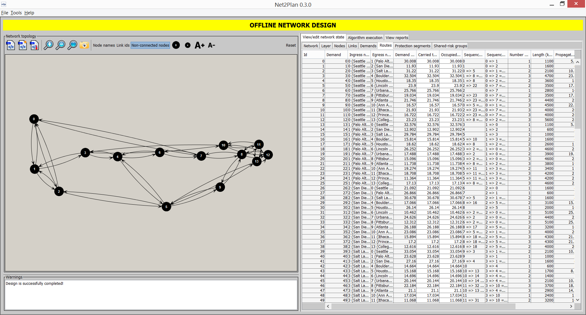
Routes (only source routing)
This sub-tab shows the information related to the routes in the network (see Section 1↑). Clicking on each route highlights its associated path in the left panel. In the sub-tab, Route Id column is a serial number starting from 0 identifying the route. Demand is the identifier of the demand associated to the route (the route carries traffic of one and only one demand). Ingress and egress node are the initial and end node of the route, that must match those of the demand. Demand offered traffic informs about the total offered traffic of the associated demand. Carried traffic is the amount of traffic carried by this route. The columns sequence of links and sequence of nodes describe the path followed by the route. The length in km sums the lengths of the links in the route. Bottleneck utilization indicates the highest utilization among the links in the route. Backup segment shows the identifiers of the protection segments associated to this route. Finally, the last column shows the user-defined key-value attributes attached to the route.
Figure 5.16 Routes view
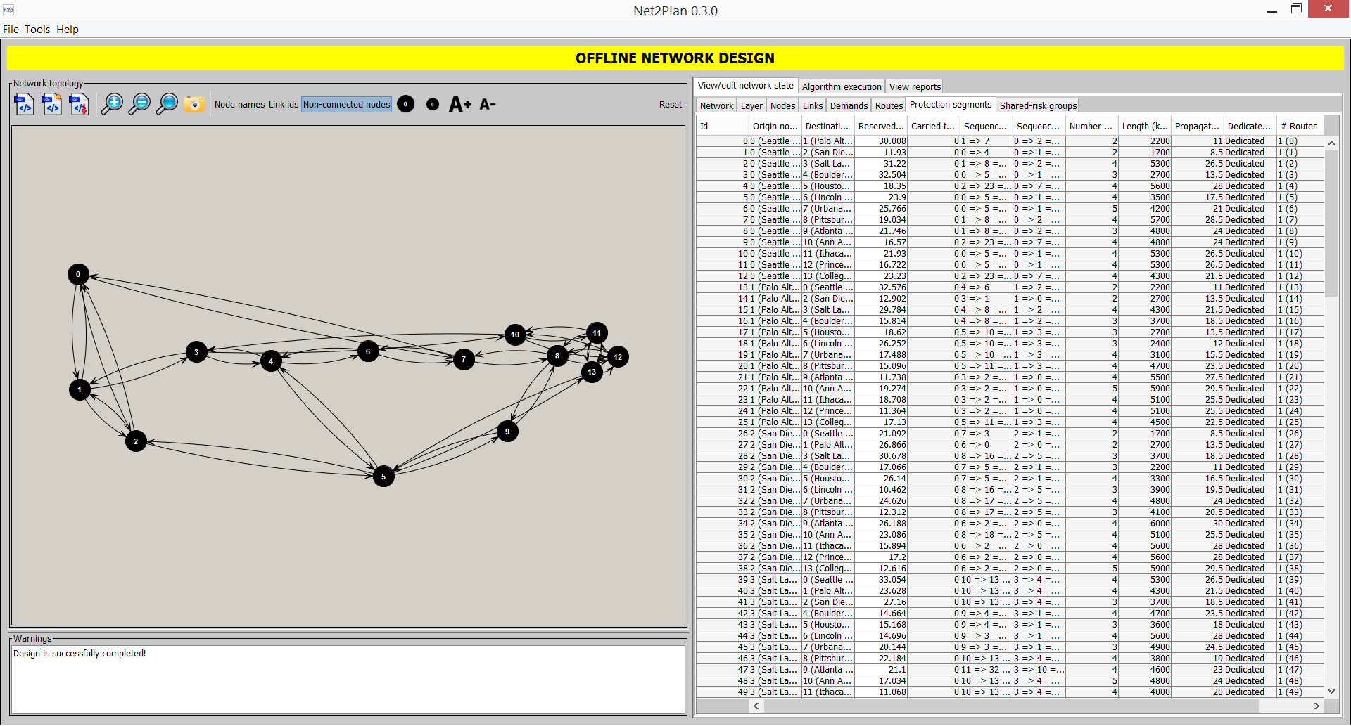
Protection segments (only source routing)This sub-tab shows the information related to the protection segments defined in the network (see Section 2↑). Clicking on each segment highlights its associated path in the left panel. In the sub-tab, Segment Id column is a serial number starting from 0 identifying the protection segment. Origin and destination node are the end nodes of the protection segment. Both nodes should be part of the route or routes that the protections segment is protecting. Reserved bandwidth is the amount of bandwidth that the segment reserves in each traversing link. The sequence of links and nodes describe the path followed by the segment. The segment length sums the lengths of the links in the path. The segment is tagged as dedicated, when it is assigned to protect only one route. Otherwise, it is tagged as shared. The #Routes column indicates the number of routes this segment is associated to, and their identifiers. Finally, the last column shows the user-defined key-value attributes attached to the protection segment.
Figure 5.17 Protection segments view
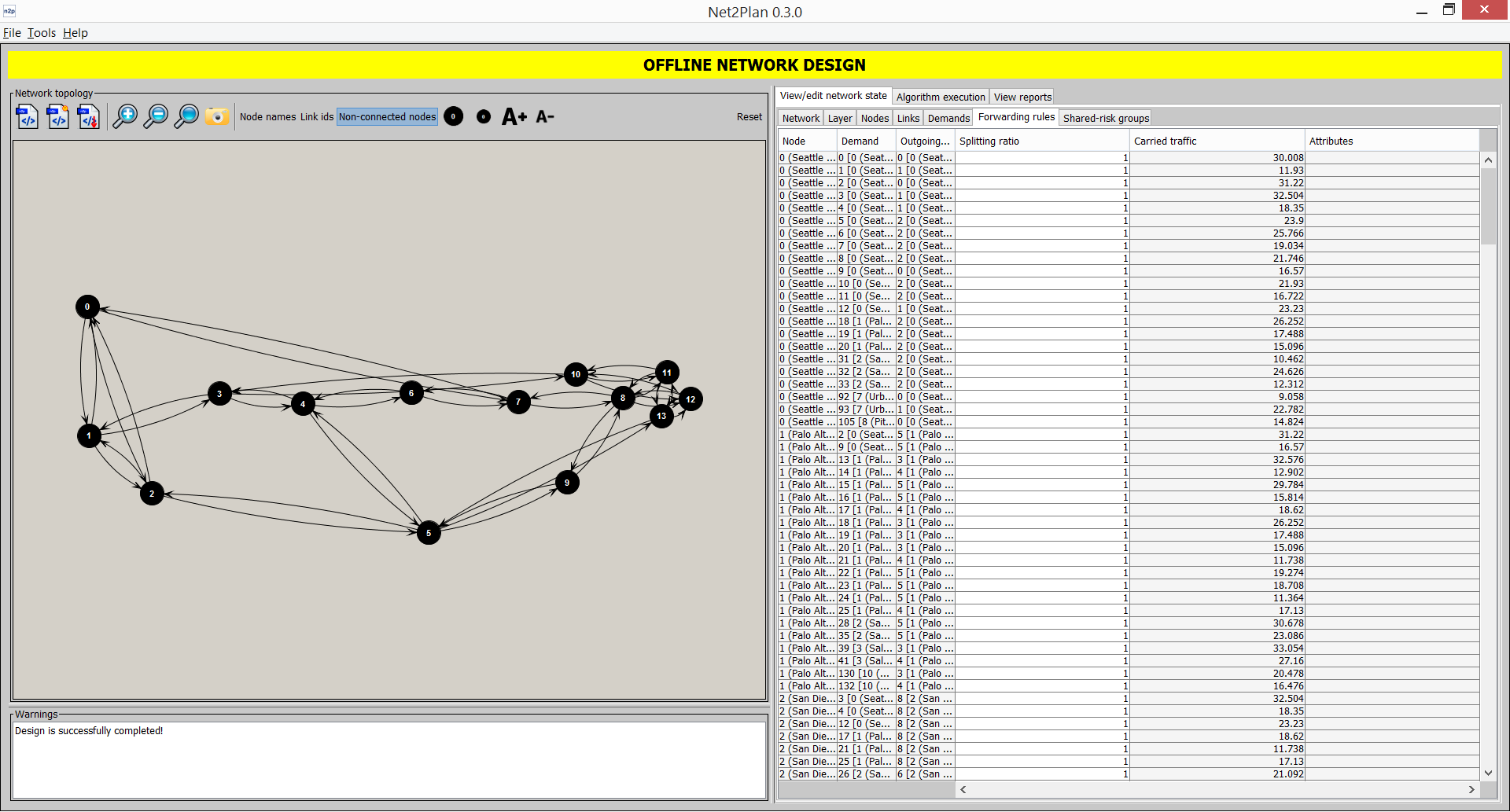
Forwarding rules (only hop-by-hop routing)
This sub-tab shows the information related to the forwarding rules defined in the network (see Section 2↑). Clicking on each segment highlights its associated path in the left panel. In the sub-tab, Segment Id column is a serial number starting from 0 identifying the protection segment. Origin and destination node are the end nodes of the protection segment. Both nodes should be part of the route or routes that the protections segment is protecting. Reserved bandwidth is the amount of bandwidth that the segment reserves in each traversing link. The sequence of links and nodes describe the path followed by the segment. The segment length sums the lengths of the links in the path. The segment is tagged as dedicated, when it is assigned to protect only one route. Otherwise, it is tagged as shared. The #Routes column indicates the number of routes this segment is associated to, and their identifiers. Finally, the last column shows the user-defined key-value attributes attached to the protection segment.
Figure 5.18 Forwarding rules view
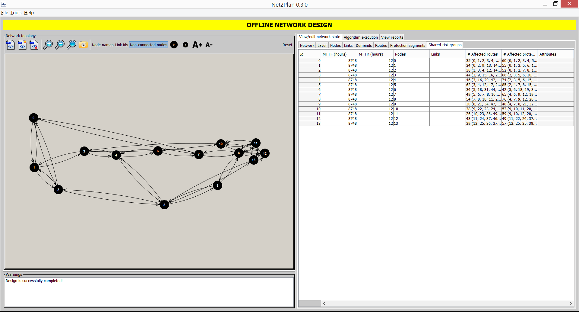
Shared-risk groups
This sub-tab shows the information related to the shared-risk groups (SRGs) defined in the network (see Section 3.1.7↑). Clicking on each SRG highlights its associated nodes/links in the left panel (the nodes and links that simultaneoously fail, if the failure event represented by the SRG occur). In the sub-tab, SRG Id column is a serial number starting from 0 identifying the SRG. MTTF and MTTR columns show the mean-time to fail and mean time to repair information in hours, that statistically characterize the occurrence of failures and the duration of repairment periods. “Nodes” and “Links” columns shows the identifiers of the nodes/links affected by the failure. The #Affected routes column indicates the number of rge routes affected by the failure, and their identifiers. Finally, the last column shows the user-defined key-value attributes attached to the SRG.
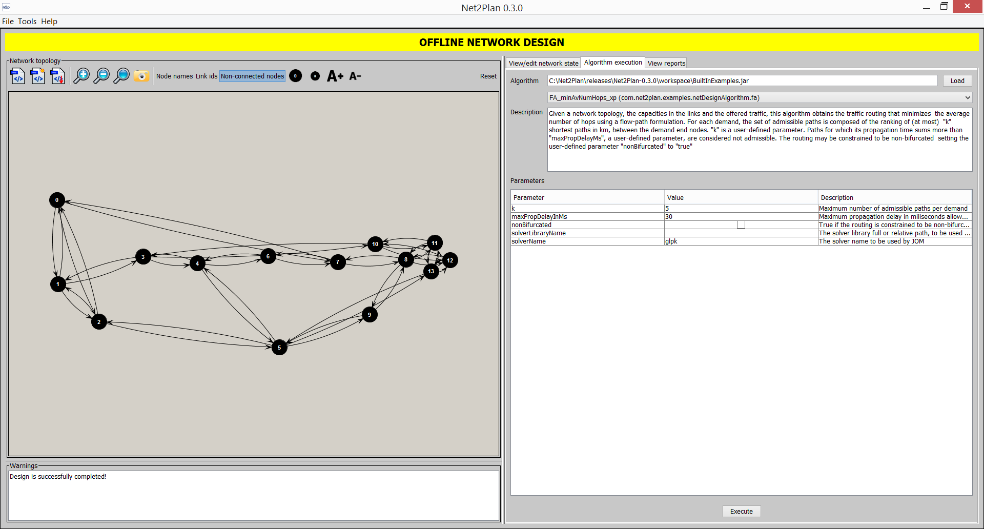
This panel (accessible also from CTRL+2) permits the users executing network design algorithms that receive as input the current network design, algorithm-defined parameters, and Net2Plan-wide parameters, and produce an output a new network design that becomes the current one, and an output message string.
To execute an algorithm, users shoud specify the Java class (implementing the IAlgorithm interface) containing the network design algorithm. A .class file can be selected using the Load button. In addition, a .jar file can be also selected. In that case, the pull-down menu below permits the user selecting one among the .class files in the .jar, that implement the IAlgorithm interface. Once an algorithm is selected, the Description text field shows the algorithm description as returned by the getDescription() method of the algorithm. The Parameters panel shows the set of input parameters of the algorithm. Net2Plan invokes the getParameters() method of the algorithm to obtain the list of input parameters, and a name, a default value, and a description message for each. This information is displayed in the Parameters panel. The graphical interface permits the user modifying the value of the parameter. The algorithm is executed pressing the Execute button. At this moment, Net2Plan invokes the executeAlgorithm() method of the algorithm, passing as inputs the current network design, the values of the input parameters (as String objects, any parsing should be done by the algorithm), and the current values of the Net2Plan-wide parameters (see 5.1.1.1↑). The executeAlgorithm() method returns a NetPlan object that becomes the current network design. If the method raises an Exception, a message is shown and the current network design is unchanged.
To see more information about how to develop user-made offline network design algorithms see the Section 5.2.6↓.
Important: To enforce reuse of single-layer algorithms in multilayer networks, as mentioned in Section 3.1.2↑, the GUI will select as default layer the one being shown at the time of execution of the algorithm.
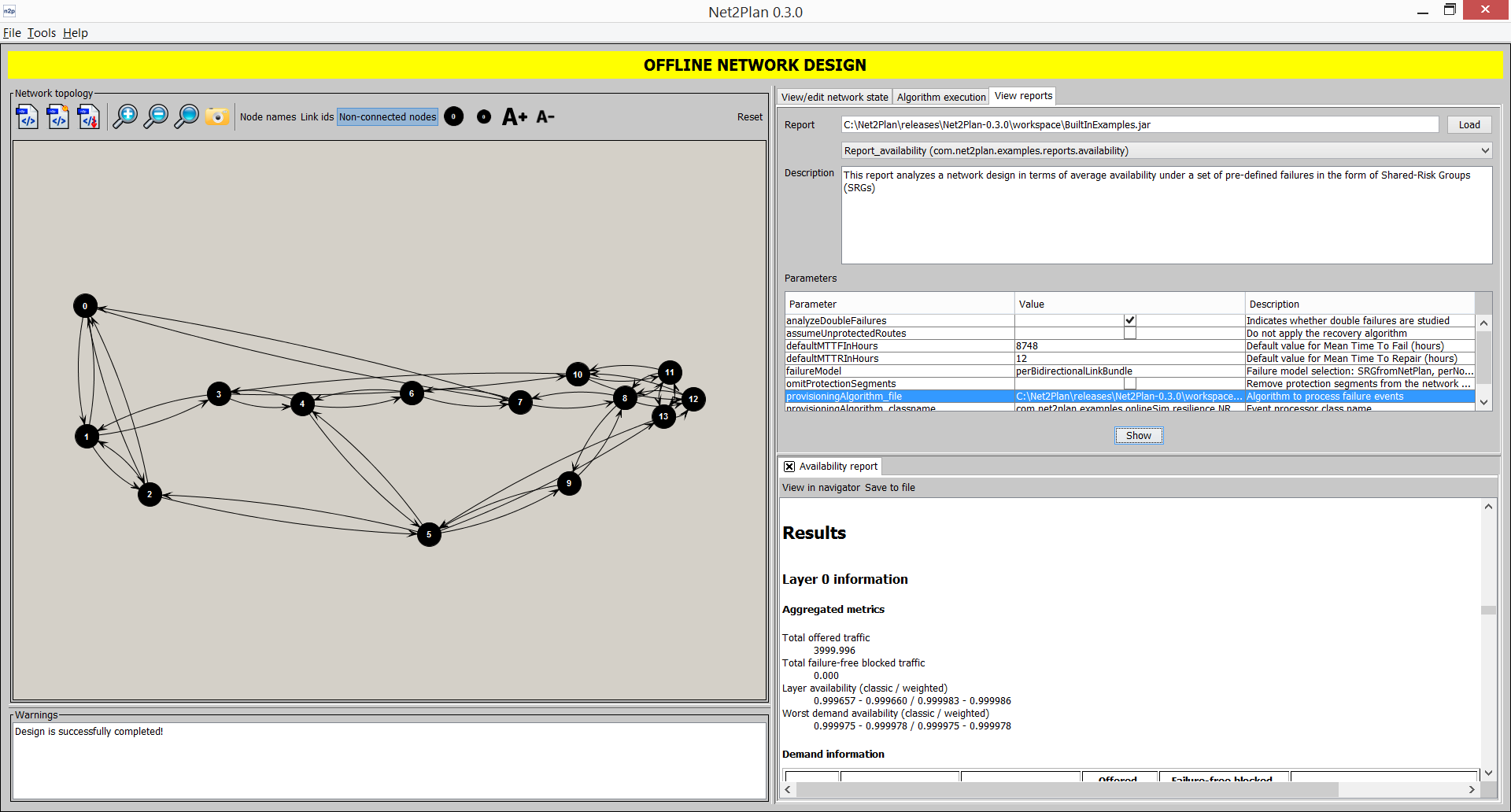
In this panel (accessible from CTRL+3) users can select a report to apply to the network plan. The structure is similar to those to execute algorithms. Upon selection and clicking Show the report is shown in the bottom part. Users can see it in a browser using the option View in navigator, or even saving to an external HTML file.
Figure 5.21 Showing a report
Reports can be closed individually using the CTRL + W combination.
5.2.6 How to build an offline network design algorithm
Users can develop their own offline network design algorithm to be executed in Net2Plan. An offline network design algorithm should be implemented as a Java class implementing the interface com.net2plan.interfaces.networkDesign.IAlgorithm. The user must implement the three methods of the interface:
String executeAlgorithm(NetPlan netPlan, Map<String, String> algorithmParameters, Map<String, String> net2planParameters): This method will be called by Net2Plan when the user clicks the “Execute” button in the graphical interface. The method receives as input parameters (i) the netPlan object containing the current network design, (ii) the values assigned by the user in the graphical interface to the algorithm parameters, (iii) the values of the Net2Plan global configuration options (see 5.1.1.1↑). The user’s code is responsible of reading and parsing the values of the input parameters (they are received as strings). Any changes that the algorithm wishes to make to the current network design, should be performed using the appropriate methods in the netPlan object received. When the algorithm ends, the user returns a message that is printed in the graphical interface, and the netPlan object becomes the new current network design. If the algorithm raises an exception, any changes performed to the netPlan do not affect the current network design, that remains unchanged.
String getDescription(): This method should produce a description message of the algorithm. The method will be called by Net2Plan when the user selects the algorithm to be executed, and the String received is shown in the graphical interface.
List<Triple<String, String, String>> getParameters(): This method should produce a list with the definition of the input parameters that the algorithm will receive. Each parameter definition is composed of three strings: (i) the name of the parameter, (ii) the default value of the parameter, (iii) a description message of the parameter. This method will be called by Net2Plan when the user selects the algorithm to be executed. The definition of the parameters received, is used to create the Parameters panel in the graphical interface, that permits the user setting the values of the input parameters, that will be passed to the algorithm when executed.
It is possible to define type-specific parameters if the default value is set according to the following rules (but user is responsible of checking in its own code):
If the default value is #select# and a set of space- or comma-separated values, the GUI will show a combobox with all the values, where the first one will be the selected one by default. For example: "#select# hops km" will allow choosing in the GUI between hops and km, where hops will be the default value.
If the default value is #boolean# and true or false, the GUI will show a checkbox, where the default value will be true or false, depending on the value accompanying to #boolean#. For example: "#boolean# true" will show a checkbox marked by default.
If the default value is #algorithm#, the GUI will prepare a new interface to select an algorithm as parameter. Three new fields will be added, including "_file", "_classname" and "_parameters" suffixes to the indicated parameter name, refer to the .class or .jar file where the code is located, the class name, and a set of parameters (pair of key-values separated by commas, where individual * key and value are separated with an equal symbol. The same applies to reports (#report#), * event generators (#eventGenerator#) and event processors (#eventProcessor#).
As stated in Section 3.1.5↑, network design contains a set of traffic demands, representing the offered traffic in the network. Each demand is characterized by an ingress and egress node, and a traffic volume representing an average of the traffic load of the demand. In ocasions, the set of traffic demands is composed of one demand for each node pair. That is, there are no two traffic demands with the same ingress and egress nodes. In these cases, it is possible to represent the demand set using a compact matrix representation, so-called traffic matrix. A traffic matrix for a network of nodes is a matrix with zeros in the diagonal. The coordinate in the -th row and -th column of the matrix, contains the amount of traffic generated in node that is targeted to node . In other words, the traffic volume of the demand associated with the node pair.
The traffic matrix design tool (see Section 5.3↑) assists users in the process of generating user-defined traffic matrices. It permits generating new matrices manually, or following several models found in the literature (e.g. random-uniform, population-distance models...). Created matrices can be saved in .n2p format to be further applied in Net2Plan. In addition, traffic matrix generation models are available in the Net2Plan library and thus can be directly integrated into Java-based design algorithms. For more information, see the class com.net2plan.libraries.TrafficMatrixGenerationModels in the Javadoc.
Selecting Traffic matrix design under Tools menu (or using ALT+2) activates the Traffic matrix design window. Fig. 5.22↓ displays the workspace window for this option. The upper part of the left window gives access to a set of general traffic generation models. Below, the user can generate matrices using one particular method: the population-distance traffic model. The right panel shows the traffic matrices generated, and permits saving (as .n2p), loading (as .n2p), resizing the matrices and some other simple modifications in the buttons above the matrices. In the lower right side, the traffic normalization panel permits applying a normalization method to one or all of the traffic matrices in the upper panel. The panel below, permits selecting a method for producing a set of traffic matrices from a seminal one, in different forms.
In this panel, the user can generate one or a batch of traffic matrices, selecting one of the following traffic generation patterns:
Constant: Generates a ( number of nodes) traffic matrix with a given constant value in all its coordinates.
Uniform : Generates a ( number of nodes) traffic matrix with random values in the range .
Uniform : Generates a ( number of nodes) traffic matrix with random values in the range .
50% Uniform & 50% Uniform : Generates a (number of nodes) traffic matrix with 50% of its entries with random values in the range , and the rest of the entries with random values in the range .
25% Uniform & 75% Uniform : Generates a (number of nodes) traffic matrix with 25% of its entries with random values in the range , and the rest of the entries with random values in the range .
Gravity model: Generates a (number of nodes) traffic matrix according to the gravity model. The user should provide for each node , its total traffic generated and received . Naturally, the sum of all the traffic generated by all the nodes should be equal to the sum of the traffic received by all the nodes (we denote it as ). From this information, the coordinate of the traffic matrix is given by . Then, the traffic from node to node is proportional to the total traffic produced at and proportional to the total traffic received at .
In any method, diagonal values of the traffic matrix are always zero, since self-demands are not allowed. Pressing the Apply button, one traffic matrix is created, and shown in the right panel. In its turn, the Apply batch button permits creating an arbitrary number of matrices, which are also shown in the right panel.
Figure 5.23 Uniform traffic models
5.3.2 Traffic generation: population-distance traffic model
In this panel, the user can generate one or a batch of traffic matrices, using the population-distance traffic matrix model described in [3]. This model receives as an input the number of nodes in the network, and for each node, its (X,Y) position, its population and a factor called node level. This information can be introduced manually in the Topology information panel, or loaded from a .n2p file, where the nodes have the population and level attribute defined.
In the population-distance model, the traffic from node to node is calculated following the expression:
where is a two-dimensional matrix (: number of levels or node types defined by the user). The level matrix allows us to e.g. introduce asymmetric traffic in the traffic generator; is the population of the node ; is the maximum population; is a matrix (: number of nodes) with the distances between nodes; is the maximum distance.
Random factor: This random factor is controlled by the input parameter , that tunes the amount of randomicity in the model. If the factor is always equal to 1, and the coordinates in the traffic matrix are not random. If , the factor equals to , and thus is a uniform random variable in . Intermediate values of yield to uniform random variables in the range
Node level factor : This factor permits multiplying the traffic between two nodes by a constant dependent on the level of each node. The values are defined in a matrix (being : number of levels or node types defined by the user). For instance, imagine we have a network with two types of nodes, “clients” and “servers”. We want to create a traffic matrix for this network where clients do not send traffic to clients, and servers do not send traffic to servers. This can be done defining two node levels in the network for separating “client nodes” and “server nodes”. Then, we can use a level matrix with 0s in the diagonals, so the client-client traffic and server-server traffic is multiplied by 0 in the model.
Population factor : The population factor makes the traffic between two nodes proportional to the product of the population of both nodes divided normalized by the maximum node population . The factor is used to smooth the effects of the product (e.g. if a population is 0, the traffic is still not zero). The factor controls the effect of the population in the matrices. Typical values are:
in models based on so-called gravitation attraction.
if site traffic is independent of population.
Distance factor : The distance factor makes the traffic between two nodes inversely proportional to the distance between them. The , and values have a similar function as in the population factor. is to avoid any possible division by 0. Typical values are:
in models based on so-called gravitation attraction.
in models based on so-called magnetism.
Note that the population and/or distance normalization factors can be also disabled.
Pressing the Apply button, one traffic matrix is created, and shown in the right panel. In its turn, the Apply batch button permits creating an arbitrary number of matrices, which are also shown in the right panel.
The right panel shows the traffic matrices generated by any of the previous models, in different tabs numbered as TM0, TM1... The user can manually modify the matrices directly typing the coordinate values. The “Resize this” button permits resizing (changing the number of nodes) of the traffic matrix in the active tab. The “Resize all” button permits resizing all of them in one step. The “Load” button permits loading a traffic matrix from a .n2p file. The buttons “Save this” and “Save all” permits saving the traffic matrix in the active tab, or all the traffic matrices in .n2p files. The buttons “Make symmetric this” and “Make symmetric all” produces symmetric matrices. The traffic between two nodes becomes the average between the traffic in both directions. The buttons “Reset this” and “Reset all” sets 0s in all the coordinates of active/all matrices. The button “Clear all” eliminates all the matrices. The button “Sum all” adds a new traffic matrix to the panel, which is the sum of all the traffic matrices shown (all of them must have the same number of nodes). The buttons “Multiply this” and “Multiply all” permits multiplying all the coordinates of this/all matrices by a constant factor.
The traffic normalization pull-down menu in the lower-right side of the window, permits selecting a normalization method to apply to the traffic matrix in the active tab (button “Apply”) or to all the traffic matrices (button “Apply all”). Four types of normalization methods are implemented: total, row and column normalization [3]. The first adjusts the traffic matrix so that the total traffic offered to the network matches a user defined value. The second (third) modifies the matrix so that the -th row (column) of the matrix sums , being () a vector defined by the user. Note that this means that the total traffic transmitted (received) by node is fixed to exactly . More formally:
Total normalization: The target of total normalization, is modifying a traffic matrix , so that in the normalized matrix , the total amount of traffic generated equals a matches a user-defined value . This is done by multiplying all the elements of the original traffic matrix by a constant factor according to the expression:
Row normalization: The target of row normalization, is modifying a traffic matrix , so that in the normalized matrix , the total amount of traffic generated by each node , equals a user-defined value . This is done by multiplying all the elements in the -th row of the original traffic matrix by the same constant factor according to the expression:.
Column normalization: The target of column normalization, is modifying a traffic matrix , so that in the normalized matrix , the total amount of traffic received by each node , equals a user-defined value . This is done by multiplying all the elements in the -th column of the original traffic matrix by the same constant factor according to the expression:.
Normalize to maximum traffic that can be carried: The target is to multiply the traffic matrix by a constant factor so that the normalized matrix , is the largest traffic matrix that can be carried by a particular network using the optimum routing (without oversubscribing the links). The user can choose between two forms of calculating this: an estimative method, and an exact method:
Estimative method. This method actually produces a matrix which is an upper bound to the maximum traffic that an optimal routing could carry. For each input/output pair in the network , it calculates the number of hops that the shortest path (either in hops or in km) between those nodes has . For each node pair , the quantity is the minimum possible amount of link bandwidth that the traffic between those nodes could consume in any routing. Then, the normalized matrix is such that the sum of this quatity along all the coordinates, equals the total amount of bandwidth summing the links in the netowork . In other words: . Note that this may produce a traffic matrix larger than what any routing could carry.
Exact method. This method solves the linear program that exactly computes the maximum factor for which the matrix still has a feasible routing in the network. The formulation is solved using the JOM library. The solver used and its .DLL/.so location is obtained from the default values in the Options menu (see 5.1.1.1↑).
Figure 5.25 Traffic normalization
5.3.5 Creating a set of traffic matrices from a seminal one
In some occasions, network design studies require a set of traffic matrices, instead of a single one. For instance, when we need to produce a sequence of traffic matrices that reflect the forecasted traffic in following years, according to a expected traffic growth. Also, it may be neccessary to produce random variations of a single traffic matrix, to check how the network performances vary if the traffic fluctuates. For this or other purposes, Net2Plan offers the following methods:
New matrices with a compound annual growth rate:A sequence of traffic matrices is created, representing one for each of the incoming years, being the seminal matrix the traffic today. Each matrix is equal to the matrix of the previous year, multiplied by a factor , where CAGR is the Compound Annual Growth Rate.
Uniform random variations: A set of matrices is created from a seminal one. For each new matrix, each coordinate is given by a sample of a uniform random variable with average (the coordinate value in the seminal matrix), and a user-defined maximum relative variation (in the range [0, 1]). For instance, a value 0.2 of the maximum relative variation means that the new coordinate is taken uniformly between and .
Gaussian random variations: A set of matrices is created from a seminal one. For each new matrix, each coordinate is given by the same coordinate in the seminal matrix, plus a sample of a gaussian random variable, with average (the coordinate value in the seminal matrix), and a user-defined coefficient of variation (quotient between standard deviation and average), and a user-defined maximum relative variation. This latter value is used to truncate the sample. For instance, a value 0.2 of the maximum relative variation means that if the sample is below then the value is produced, and if the sample is greater than , the value is produced. Finally, if the sample is below 0, the coordinate is set to 0.
In a real-world environment, network conditions vary during its operation, according to different phenomena. Failures in nodes and links, establishment of new virtual circuits, or variation in traffic volumes are some examples. In this case, users could be interested in analyzing, using an event-driven simulation, how their networks react to those changes and how their designs are consequently adapted for it.
Net2Plan provides a post-analysis simulation tool that allows user the (joint) evaluation of the availability performance of protection and restoration algorithms in the network, the performance of on-line provisioning schemes that allocate resources to incoming connections (e.g. virtual circuits requests, lightpath requests, phone calls, multimedia sessions), or the performance of dynamic allocation algorithms which react to variations in traffic demand volumes. Allocation is not only referred to modify traffic routing, but also it means that the network topology may change along time (e.g. adding new links, updating the link capacities...) for adapting to the new traffic condition.
The architecture of the simulator is based on the well-known discrete-event simulation paradigm. The network operation is modeled as a discrete sequence of events in time. Each event occurs at a particular instant in time and marks a change of state in the system [10]. Between consecutive events, no change in the network occurs; thus the simulation can directly jump in time from one event to the next.
The basic event-driven simulation model is explained next. The Event generator creates events according to a given algorithm (built-in or user-made), and deposits the ordered events (i.e. “a failure will happen at X seconds in simulation time”) in the event list in the Kernel. Then, the scheduler in the Kernel steps through the event list in chronological order according to the global simulation time clock, sending the event to the Event generator to process the event (i.e. to provoke the failure), directly modifying the network stat. This will generate a new notification event (i.e. “a failure happened”) that will be added to the event list. Finally, the Event Processor (which can also be user-made) will be called to take some reactions. Statistics are collected by the Kernel during the simulation after each event. An interesting feature of the online simulator is that the event generator and the event processor can send events between them, and also to themselves. As mentioned, the typical interaction is sending events from the generator to the processor, e.g. conveying failure/reparation notifications. However, self-events permit simulate e.g. the effect of a “hold-off” timer in multilayer networks or the delay in failure detection.
Regarding to the statistics collection, Event generator and Event processor provide a method so-called finish, which is called when the simulation ends, and can be used to print technology-specific statistics that the algorithm (not that ones that the Kernel may have collected). For more information about implementation details check the com.net2plan.interfaces.simulation package in the Library API Javadoc.
Selecting Online simulation (also from ALT+3) opens the corresponding window. The workspace of the window is divided into three areas, in a similar way to the network design mode: data input and visualization (top-left area), execution and reporting (right area), and simulation controller and information area (bottom-left area). Actually, the interface is an extension of the offline network design tool, with three basic differences: (i) users cannot modify manually the design in the “View network state” tab, (ii) users should incorporate an event generator (extending the base class IEventGenerator) and an event processor (extending the base class IEventProcessor) instead of a design algorithm in the “Execution controller” tab, and (iii) after finishing the simulation a report with some metrics (including either predefined or own-developed metrics) is shown in “Simulation report” tab.
As for network design, this panel is used for graphically design and see networks. In contrast, here users cannot directly modify the topology. To do so, the Offline Network Design tool must be used. In order to perform a simulation, a network design must be loaded. The content of the design is dependent on the requirements of the event generator and processor.
During the simulation, changes in the topology (i.e. failed nodes and/or links) will be shown in the canvas (this will be explained in the next section).
In the View network state tab (accessible also from CTRL+1), users can see information related to the network state. Optionally, users can also see the same information (gray-shaded) as it was in the base network design before running the simulation, for comparisons.
Figure 5.28 View network state for a path restoration algorithm (links in red are failed links, links with dashed lines are the primary path, and the ones with complete lines are the current ones)
With this panel, users are able to execute simulations and view the current state of the network. In the Execution controller (accessible also from CTRL+2), users can load network designs and execute simulations. To execute a resilience simulation the user should specify the following things:
Simulation parameters: general parameters for the simulation.
“disableStatistics”: In some occasions, users might be interested in collecting only their own statistics, and would prefer avoiding the overhead that requires statistics collection by the Kernel. This can be done with this parameter. In this case, kernel statistics will present zero-valued results, while algorithm-specific statistics are shown. Allowed values are “true” or “false”.
“omitProtectionSegments”: As stated in Section 2↑, protection segments reserve a certain amount of bandwidth to provide (partial) backup-paths for primary routes. However, in some situations, users might be interested in executing their simulations assuming that no protection segments are defined. If this parameter is set to true, then protection segments are removed from the network plan just before the simulation starts, and their bandwidth in the links is available for carrying common routed traffic. Allowed values are “true” or “false”.
“refreshTime”: If the option “Refresh” has been activated in the simulation controller panel, information about the current simulation, (number of processed events, simulation and cpu time...) will be shown there. This information will be refreshed every number of seconds given by this parameter. Allowed values are integers greater than 0.
“simEvents”: Total number of events (including transitory events) to be simulated. If the parameter “simTime” is also specified, the simulation will automatically finish when the first stopping condition is met. Allowed values are integers greater than zero, or -1 for no limit (simulation must be manually stopped).
“simTime”: Total simulation time (including transitory events) in seconds. If the parameter “simEvents” is also specified, the simulation will automatically finish when the first stopping condition is met. Allowed values are integers greater than zero, or -1 for no limit (simulation must be manually stopped).
“transitoryEvents”: Number of events for the transitory period. If “transitoryTime” is also specified, the transitory period will finish when the first condition is met. Allowed values are integers grater than 0, or -1 for no transitory period.
“transitoryTime”: Transitory time in seconds. If “transitoryEvents” is also specified, the transitory period will finish when the condition is met. Allowed values are integers greater than 0, or -1 for no transitory period.
Event generator: the event generator algorithm, as a Java class extending the IEventGenerator class. This is the class in charge of generating events. Net2Plan includes several algorithms, but others can also be implemented and loaded by the user (using the Load button). A description of the algorithm will be show in this panel as well as any input parameter thay may be modified by the user.
Provisioning algorithm: the event processor algorithm, as a Java class extending the IEventProcessor class. This is the class in charge of reacting to events. Net2Plan includes several algorithms, but others can also be implemented and loaded by the user (using the Load button). A description of the algorithm will be shown in this panel as well as any input parameter that may be modified by the user.
Algorithms can be loaded as .jar or .class files. More information about user-made algorithms can be found in the Library API Javadoc.
During the simulation, users are able to save the current network state (tanslated into a network plan) using the corresponding button in the network topology view.
Figure 5.29 Execution controller view
Important: Once the simulation is started, none of the above options can be changed. Users should stop and resetthe simulation (clicking the Reset button) to perform changes.
In this panel users can control the execution and flow of the simulation. Several buttons can be manipulated here:
Run: This button will start the simulation. Information about the current simulation will be shown in the text panel (the refresh time is defined by the “refreshTime” parameter). If a previous simulation has already been started it must be stopped and reset before starting a new one.
Step: Instead of running continuously, the simulation can be advanced in steps.. Each time the “Step” button is clicked the simulation will consume one event of the future event list, and then pause and refresh the text panel.
Pause/Continue: The simulation will be paused or resumed each time this button is clicked. A simulation must be started in order for this button to work.
Stop: Users can stop the simulation at any time, but then the simulation cannot continue.
Refresh: The information in the text panel will be refreshed if this check-box is activated.
View FEL: Clicking this option will show the Future Event List, where users can examine the future events to be processed by the provisioning algorithm:
Figure 5.30 Future Event List (FEL)
Also, the text panel shows some brief simulation state information: simulation time, CPU time, last event processed... This information is updated according to the refresh time parameter.
In this panel (accessible also from CTRL+3), users can obtain the availability statistics collected by the kernel, and also those collected by their algorithms (event generator and event processor). Users can see the report at any moment (clicking the Update button) while the simulation is running, paused or stopped, and can be opened by a web browser, as happened with the reports for network designs.
In some occasions, users might be interested in collecting only their own statistics, and they might want to eliminate the (large) overhead that requires statistics collection. This can be done by setting the simulation parameter “disableStatistics” to “true”. In this case, kernel statistics will present zero-valued results, while algorithm-specific statistics are shown.
Report shows different network-wide, per-layer, per-node, per-link and per-demand information. Algorithm-specific information can be included via the finish method of IEventGenerator and IEventProcessor classes.
Similarly to the reporting tool (accessible also from CTRL+4) into network design, users can select a report to apply to the current network state. Upon selection and clicking Show the report is shown in the bottom part. Again, reports can be opened by a web browser using the option View in navigator.
Contrary to the GUI, the command-line interface allows users to make use of batch processing or large-scale simulation features, thus it is specifically devoted to in-depth research studies. As stated before, all features available for GUI mode are also available here.
The execution is controlled via command-line arguments. To run Net2Plan in CLI mode, users must execute the following command in a terminal:
java -jar Net2Plan-cli.jar [more options]
Help information can be obtained through the help argument in the following ways:
To obtain a brief information, including only the execution modes, users should execute the CLI without arguments: java -jar Net2Plan-cli.jar
To obtain the complete information, including individual help for every execution mode, users should execute: java -jar Net2Plan-cli.jar --help
To obtain the information about a certain execution mode, users should execute: java -jar Net2Plan-cli.jar --help mode-name
Then, help for the selected mode is shown. All commands and options are self-explained there.
Anyway, we show here some examples:
To execute the FA_shortestPath algorithm for the NSFNet network and its reference matrix: java -jar Net2Plan-cli.jar --mode net-design --input-file workspace\data\networkTopologies\NSFNet_N14_E42.n2p --traffic-file workspace\data\trafficMatrices\NSFNet.n2p --output-file workspace\data\NSFNet.n2p --class-file workspace\BuiltInExamples.jar --class-name FA_shortestPath --alg-param shortestPathType=km
To execute the network design report over the previous design: java -jar Net2Plan-cli.jar --mode report --input-file workspace\data\NSFNet.n2p --output-file workspace\data\report.html --class-file workspace\BuiltInExamples.jar --class-name Report\networkDesign
To generate a series of 4 10x10 traffic matrices using a (0, 100) random uniform model: java -jar Net2Plan-cli.jar --mode traffic-design --num-nodes 10 --traffic-pattern uniform-random-100 --output-file workspace\data\trafficMatrices\tm10nodes.n2p --num-matrices 4
Important: To avoid excessive verbosity in the CLI, package names for Java classes can be omitted. Note that in case of .jar files the first class matching the class name will be selected, in case multiple cases in different packages share the same class name.
Important: Restrictions to the path of .class files must follow the guidelines in Section 3.2↑.
New: A new plugin architecture (undocumented) has been created to support the integration of external CLI/GUI tools or I/O filters. Original plugins are dettached from kernel and are also located into plugins folder
Net2Plan 0.3.0 (June 29, 2015)
Major changes in network model:
New: Complete multilayer support, including layer coupling (links at an upper layer become demands at a lower layer, or viceversa)
New: Identifiers for nodes, links, demands, and so on, are now long values. get() methods, whose output were arrays, now return maps
New: Internal speed-up via caching of common get() methods
New: ’Online simulation’ is a new tool that merges the previous simulators into a common one, and it uses the same network model than for network design
Improved documentation
Net2Plan 0.2.3 (March 7, 2014)
Minor changes
Improved documentation
Net2Plan 0.2.2 (October 16, 2013)
Minor changes
Improved documentation
Net2Plan 0.2.1 (May 23, 2013)
New: ’Time-varying traffic’ simulator
New: ’Network design’ is now able to execute multilayer algorithms
Minor changes
Net2Plan 0.2.0 (March 18, 2013)
Initial Java version, many major changes from latest MATLAB version
In its very early stage Net2Plan was designed as a MATLAB toolbox. From version 0.2.0, previous MATLAB versions were discontinued, thus backward-compatibility is not ensured at all. However, interested users can found them in the website.
Net2Plan tool has its origins in 2011, during the preparation of the teaching materials for two new Communication Networks Planning courses at Universidad Politécnica de Cartagena (Spain) taught by Prof. Pablo Pavón Mariño:
“Telecommunication networks theory” (2nd year, 2nd quarter, “Degree in Telematics Engineering” and “Degree in Telecommunication Systems Engineering”
“Network planning and management” (3rd year, 2nd quarter, “Degree in Telematics Engineering”)
Net2Plan is also a part of the Ph.D. work of José Luis Izquierdo Zaragoza, supervised by Prof. Pablo Pavón Mariño.
Aside from Net2Plan, authors also collaborate in the development of MatPlanWDM, an open-source tool for multilayer optical networks. In addition, Prof. Pablo Pavón Mariño develops JOM (Java Optimization Modeler), an open-source Java library for modeling and solving optimization problems in a simple MATLAB-like syntax.
[3] Robert S. Cahn. Wide area network design: concepts and tools for optimization. Morgan Kaufmann Publishers Inc., 1998.
[4] A. Girard. Routing and dimensioning in circuit-switched networks. Addison-Wesley, 1990.
[5] Iyad Katib, Deepankar Medhi. IP/MPLS-over-OTN-over-DWDM Multilayer Networks: An Integrated Three-Layer Capacity Optimization Model, a Heuristic, and a Study. IEEE Transactions on Network and Service Management, 9(3):240—253, 2012.
[6] Leonard Kleinrock. Queueing Systems, Volume 1: Theory. Wiley-Interscience, January1975.
[8] Pablo Pavon-Marino, Jose-Luis Izquierdo-Zaragoza. Net2Plan: An Open Source Network Planning Tool for Bridging the Gap between Academia and Industry. IEEE Network, 29(5):90—96, 2015. URL http://dx.doi.org/10.1109/MNET.2015.7293311.
[9] Pablo Pavon-Marino. Network optimization: modeling and algorithms. A hands-on approach. John Wiley & Sons, may2016.
[10] Stewart Robinson. Simulation: The Practice of Model Development and Use. Wiley, March2004.
[11] K.W. Ross. Multiservice loss models for broadband telecommunication networks. Springer, 1995.
Net2Plan defines a network representation based on abstract concepts such as nodes, links, routes, traffic demands and network layers, without relying on any network technology. This is the key idea that allows Net2Plan to not be constrained by any particular network technology, and is, thus, applicable to any and all of them. To achieve such functionality, we define a data storage called network plan (class com.net2plan.interfaces.networkDesign.NetPlan in the Net2Plan library) which contains all the current state of the network design, so every algorithm receives a network plan and returns a modified network plan.
In this section, we provide the theoretical framework that is behind Net2Plan philosophy, and the (common) notation we use to characterize the network, topology, routing, etc. For a more detailed explaination, see [9].
In Net2Plan a network topology is defined as a graph , where is the set of nodes and is the set of links. The number of nodes and links are the cardinality of sets and , which are and , respectively. Network topologies are considered as multi-digraphs. This means that every link is unidirectional (directed graph or digraph), and that network topologies can have multiple links between the same node pair. No self-links are allowed.
Given a link , denotes the initial node of the link, and denotes its destination node. We use to denote the link length (measured in km). Given a node , is the set of outgoing links from () and is the set of incoming links to (). In Fig. A.1↓ an example of network topology is shown.
Figure A.1 Topology with = 3 nodes, , = 3, . End nodes of are and . Outgoing links from node are , and the incoming one is
Each link in a network has associated a real number which represents its capacity. The capacity is the amount of traffic the link is able to carry. Thus, capacities and traffics are measured in the same units. Unless stated otherwise, the traffic and capacities in Net2Plan are measured.
For the sake of simplicity, we denote the set of link capacities as a vector . In addition, the carried traffic by link is denoted by . The vector represents the traffic carried in all the links in the network.
Typically, link capacities are limited to a discrete range of values due to technological reasons, such as STM- carriers in SDH. In these cases, capacities are referred as modular capacities.
Traffic is modeled through a set of demands (or commodities) . Each demand represents an offered traffic flow to the network. In general, the traffic of a demand can have one or more ingress nodes in the set , and one or more egress nodes denoted by the set ; however, in current version of Net2Plan demands are considered unicast. This means that each demand has one ingress node and one egress node, thus . In addition, self-demands are not allowed.
The offered traffic by a demand is represented as . Note that such value may not be measured in the same units than link capacities . In some situations, it is not possible to carry all the offered traffic by the demands. Then, represents the amount of traffic belonging to demand that is carried. In their vector form, and represent offered and carried traffic, respectively.
Given a network topology , a path is an ordered sequence of links , such that the destination node of a link is the origin node of the following link . The set of all possible paths in a network is denoted as . The first node of the path is the origin node of the first link , and the last node in the path is the destination node of the last link . Finally, given a link , is the set of paths which traverse the link . For example in Fig. A.2↓, given and , . In addition, is the number of hops in path .
Figure A.2 Topology with = 4 nodes, , = 4 links,
In Net2Plan, the routing is internally represented in the form of demand-path variables. Formally, for each demand in the network, a set of paths is defined between the end nodes of the demand (, ). Also, given a path , the demand that the path is linked to is denoted as . Then, traffic routing is represented by a vector where is the traffic volume carried through the path for demand , occupying a certain amount of capacity in the links. Note that we define a path as a sequence of links that carry traffic of a specific demand . If two demands exist between the same end nodes, and the traffic of both demands is carried through the same sequence of links, we consider in Net2Plan that the routing is composed of two paths with the same end nodes, one for each demand, so that .
According to the notation used to define the network routing in Net2Plan, the following relations hold:
where Eq. ↓ implies that the traffic carried by a demand is the sum of traffics in the paths assigned to that demand, and this amount is upper bounded by the offered traffic by the demand, while Eq. ↓ reflects the fact that the traffic in a link is the sum of the traffic in the paths traversing that link, and is constrained (in general) to be limited by the link capacity.
The set of all possible protection segments in a network is denoted as . The first node of the protection segment is the origin node of the first link in the original route which is not in the protection segment, and the last node in the protection segment is the destination node of the last link which is in the original route and not in the protection segment. A link may be associated to several protection segments, which is denoted as . Finally, given a path , is the set of protection segments which protect the path . In addition, is the number of hops in protection segment .
Protection segments resemble “virtual links”, in the sense that a protection segment has a reserved capacity (greater than zero) and this capacity can be shared by several traffic routes. For example, if a protection segment has reserved 10 capacity units and a route is using 5 capacity units, still there is 5 capacity units available for other routes.
In this section several performance metrics are described. These metrics are useful to define objective functions or problem constraints. Notation is based on that presented in Appendix A↑.
Link carried traffic: It is equal to the sum of the occupied capacity of each route traversing the link
Link utilization: It is equal to the carried traffic by the link and the total reserved bandwidth by protection segments associated to the link, all divided by the link capacity
Demand carried traffic: It is equal to the sum of the carried traffic of each route associated to the demand
Link carried traffic: It is equal to the sum of the occupied capacity
Link utilization: It is equal to the carried traffic by the link divided by the link capacity
Demand carried traffic (considering that egress node does not forward its own traffic): It is equal to the sum of the carried traffic of each route associated to the demand
In packet-switched networks, traffic sources split data into smaller pieces called packets, along with a header with control information. Per each received packet, switching nodes read its header and take appropriate forwarding decisions.
In real networks, traffic is highly unpredictable and often modeled as random processes. When it is said that a traffic source generates traffic units, it is referred as average traffic. As a result, link capacities would be not enough to forward traffic and nodes have to store packets in queues, so they are delayed until they can be transmitted (this delay is known as queuing delay). If this situation remains for a long time, queues are filled and links become saturated, provoking packet drops.
Network design tries to model statistically delays and drops in order to minimize their effects. In Net2Plan each link is modeled as a queue fed by a self-similar source with a given Hurst parameter, getting the whole network average delay using Kleinrock’s independence assumption [6].
Propagation delay per link (seconds)
where is the speed of light when traverses link
Transmission delay per link (seconds)
where is the average packet length (in bits), and is the capacity in bits per second per one capacity unit
Buffering delay per link (seconds)
where Hurst Parameter. Choosing yields to same result as that predicted by M/M/1 queue model
In circuit-switched networks, traffic sources reserve a given capacity during certain time, along paths followed by traffic demands. It is possible that if a new traffic source wants to reserve resources its petition would be blocked, since it would not be enough available resources to satisfy its demand. Here, theload-sharingmodel is applied [4, 11]. According to this model, each connection request from a demand chooses randomly a path among the paths in . The probability of choosing a path is proportional to the traffic carried, and given by . After choosing the path , the connection is accepted if all the links in have enough spare capacity. If not, the connection is blocked. This means that there is no attempt to carry the connection in other possible routes in . This is the distinguishing trait of this model. Note that thanks to this assumption, there is no overflow traffic in the network (traffic offered to a route, that if blocked, and overflows to an alternate route).
It is assumed that arrivals of connection requests to each link are Poisson processes, independent link-by-link. Therefore, blocking performance metrics can be computed using Erlang-B formula. Obviously only has sense when link capacities are integer.